This document summarizes a study that examines the relationship between oil consumption and economic growth in Turkey from 1961 to 2016. It begins by reviewing previous literature on the relationship between energy use and economic growth, which has found varying results. It then describes the data and methodology used in the study, which employs autoregressive distributed lag (ARDL) modeling and Toda-Yamamoto causality testing to analyze the cointegration and causality between oil consumption and GDP in Turkey while accounting for structural breaks. The results of these analyses reveal that economic growth Granger causes oil consumption in Turkey but not vice versa, indicating that energy conservation policies would not harm economic growth.

1. Business, Management and Economics Research
ISSN(e): 2412-1770, ISSN(p): 2413-855X
Vol. 5, Issue. 6, pp: 77-85, 2019
URL: https://arpgweb.com/journal/journal/8
DOI: https://doi.org/10.32861/bmer.56.77.85
Academic Research Publishing
Group
*Corresponding Author
77
Original Research Open Access
Oil Consumption and Economic Growth in Turkey: An ARDL Bounds Test
Approach in the Presence of Structural Breaks
Özgür Özaydın*
Department of Economics, FEAS, Ondokuz Mayıs University, Samsun, Turkey
H. Alper Güzel
Department of Economics, FEAS, Ondokuz Mayıs University, Samsun, Turkey
Abstract
The aim of this study is to investigate the relationship between oil consumption and income in Turkey, using annual
data from 1961 to 2016. The stationarity properties of the series are analyzed with Lee and Strazicizh (2003), unit
root test allowing for two structural breaks, along with the conventional unit root tests namely ADF, PP and KPSS.
Due to conflicting findings of the unit root tests, ARDL bounds test approach to cointegration is used to capture the
relationship between oil consumption and income. The findings of the ARDL bounds test indicated that oil and
income are cointegrated. The causal relationship between the variables is also examined by employing Toda and
Yamamoto (1995), approach to Granger non-causality. The outcomes of the Toda and Yamamoto (1995), procedure
showed that the direction of the causality is running from real GDP to oil consumption, but not vice versa. Both
bounds test and Toda and Yamamoto (1995), test results reveal that, energy conservation policies will not harm
economic growth in Turkey.
Keywords: Oil consumption; Economic growth; Turkish economy; ARDL.
CC BY: Creative Commons Attribution License 4.0
1. Introduction
Two major oil crises stimulated by the dramatic increases in oil prices adversely affected the world economy in
1970’s. Since then, the relationship between energy use and economic growth has been a central issue for
researchers. As uncovering the relationship between energy use and economic growth may have important policy
implications regarding a country’s energy policy, many studies have been devoted to shed more light on the energy
use-income relationship. To this extend, four main types of hypotheses which reflects the possible relationships
between energy use and economic growth are tested. Growth hypothesis suggests a unidirectional relationship
running from energy use to economic growth, while conservation hypothesis also proposes a unidirectional
relationship but this time running from economic growth to energy use. According to the feedback hypothesis both
energy use and economic growth affects each other, implying that there exists bi-directional relationship between the
variables. Finally, neutrality hypothesis claims that economic growth does not lead to any significant changes in
energy use and vice versa.
Turkey is an ―energy corridor‖ between the energy exporter countries of the Middle East and the energy
importer countries of Europe due to its geographical location. As Turkey is a fast industrializing country, economic
activities in Turkey depends heavily on energy inputs. Thus, any surges in energy consumption may lead to
fluctuations in economic activity. Furthermore, changes in economic growth rates may also cause changes in
Turkey’s energy necessity. Therefore, uncovering the existence and the direction of the relationship between energy
use and economic growth for Turkey may bring important policy implications.
Since, oil has the highest share in Turkey’s energy use and Turkey is also heavily dependent on imports to meet
its oil demand, oil consumption is used as a proxy for energy use in this study. This paper aims to address the
question whether there exists a relationship between oil use and economic growth in Turkey for the period 1960-
2016. To uncover the oil use-economic growth relationship for Turkey, Auto Regressive Distributed Lag (ARDL)
modeling approach to co-integration developed by Pesaran and Pesaran (1997), and Toda and Yamamoto (1995),
causality test are employed.
The main contribution of this paper to the existing literature is taking into account the effects of structural
breaks and using the structural break dates as explanatory variables in the estimated ARDL models by using the most
recent data for the case of Turkey.
The paper proceeds as follows. A brief review of the existing literature is presented in section 2. In section 3,
the description of the data and methodology are introduced. In section 3 the empirical results obtained from the
model(s) are reported. Finally, by discussing the outcomes, policy suggestions regarding Turkey’s energy policy are
presented in section 5.

2. Business, Management and Economics Research
78
2. Literature Review
In their pioneering work (Kraft and Kraft, 1978) find unidirectional causality running from GNP to energy use
in the US for the period 1947-1974. However, Akarca and Long (1980), and Yu and Hwang (1984), suggest that
energy use and GNP to be neutral for the US, when the period covered is changed. Moreover, Yu and Choi (1985),
provide support for neutrality hypothesis not only for the US but also for the UK and Poland. On the other hand, Yu
and Choi (1985), find unidirectional causality running from energy use to income for Philippines, and income to
energy use for South Korea.
Following these seminal works, many researchers have investigated the energy use-income relationship for
different countries, over different periods and by employing different techniques. However, the results are still
contradictory. Some researchers report unidirectional causality running from income to energy use, such as,
Abosedra and Baghestani (1989), for the US, Masih and Masih (1996), for Indonesia, Soytas and Sari (2003), for
Italy and Korea, Lee (2006), for France, Italy and Japan, Zamani (2007), for Iran, Ghosh (2009), for India, Yazdan
and Hossein (2012), for Iran, Alam and Paramati (2015), for 18 developing countries, Saboori et al. (2017), for
South Korea.
On the other hand, some researchers find reverse unidirectional causality, running from energy to income, such
as; Masih and Masih (1996), for India, Stern (2000), for the US, Soytas and Sari (2003), for France, Japan and West
Germany, Oh and Lee (2004), for Korea, Lee (2005), for 18 developing countries, Soytas and Sari (2006), for France
and the US, and Yuan et al. (2007), for China, Saboori et al. (2017), for China and Japan.
Bidirectional relationship also found in some studies, such as; Erol and Yu (1987), for Japan, Masih and Masih
(1996), for Pakistan, (Glasure and Lee, 1997) for South Korea and Singapore, and Masih and Masih (1997), for
Korea and Taiwan, Hondroyiannis et al. (2002), for Greece, Ghali and El-Sakka (2004), for Canada, Soytas and Sari
(2006), for Canada, Italy, Japan and UK, Yuan et al. (2008), for China, Bhusal (2010), for Nepal, Al-Mulali (2011),
for MENA countries, Behmiri and Manso (2013), for Sub-Saharan Africa, Park and Yoo (2014), for Malaysia, Wang
et al. (2016), for China and Pinzón (2018), for Ecuador.
Despite the fact that most of the empirical studies found evidence in favor of the relationship between income
and energy use, some researchers provide evidence of energy use and income to be neutral, such as, Cheng (1995),
for the US, Masih and Masih (1996), for Malaysia, Singapore and the Philippines Cheng and Lai (1997), for Taiwan,
Glasure (2002), for Korea, Soytas and Sari (2003), for the US, the UK, Canada, Indonesia and Poland and Lee
(2006), for the UK, Germany and Sweden.
The controversy about the existence and the direction of the relationship between energy use also holds for the
studies concerning Turkey. Soytas et al. (2001), Soytas and Sari (2003), Altinay and Karagol (2005), Mucuk and
Uysal (2009), Karagöl et al. (2011), Ceylan and Başer (2014), and Keskin (2017), provide support for unidirectional
causality running from energy to income, while the findings of Lise and Van Montfort (2007), Ozata (2010),
Gokmenoglu and Taspinar (2016), and Aydin (2018), show unidirectional causality running from economic growth
to energy consumption. The validity of the feedback hypothesis is confirmed by the findings of Aktas and Yilmaz
(2008), Saatci and Dumrul (2012), and Ozturk and Acaravci (2013). In contrast to these findings, Altinay and
Karagol (2004), Soytas and Sari (2009), Ozturk and Acaravci (2010), and Ucak and Usupbeyli (2015), suggest that
energy use and income to be neutral for the case of Turkey.
3. Data, Model and Methodology
3.1. Data
Annual data for Turkey over the period 1960–2016 is used to investigate the dynamic relations between oil
consumption and income. Real GDP and total primary energy supply (TPES) from oil were used as proxies for
income and oil consumption, respectively. Real GDP is measured in US dollars (base year=2010) and oil use
measured in thousand tonnes of oil equivalent (toe). The data for the Real GDP was obtained from World
Development Indicators database of the World Bank and oil information is taken from the World Energy Statistics
and Balances of the International Energy Agency which is available at the OECD database.
3.2. Model
In order to test whether there exists a relationship between oil consumption and income the following models
are used.
(1)
(2)
where denotes time, refers to oil consumption and represents income.
The models represented with Equation 1 and Equation 2 are transformed into the following log-log models in
order to capture the long run elasticities of the variables.
(3)
(4)
where refers to time, is the log of oil consumption, is the log of income, ’s and ’s are OLS
estimators and ’s are the white noise terms.

3. Business, Management and Economics Research
79
4. Methodology
The dynamic relations between oil consumption and income are investigated by using linear time series
techniques. One of the most important problems while working with the time series data is the possibility of spurious
regression. In order to overcome the spurious regression problem, the stationarity properties of the series in question
are analyzed by using the conventional stationarity tests, which do not take into account the structural breaks,
namely Augmented Dickey Fuller (ADF), Phillips-Perron (PP) and Kwiatkowski–Phillips–Schmidt–Shin (KPSS).
Moreover, recently developed Lee and Strazicizh (2003), (LS) unit root test which allows for two structural breaks is
also employed in this study.
VAR models and residual or maximum likelihood based cointegration tests like Engel and Granger (1988),
Johansen (1988), Johansen and Juselius (1990), and Gregory and Hansen (1996a), Gregory and Hansen (1996b), are
widely used methods by the researchers to capture the inter-relations between the variables in question. Since these
methods deal only with the variables integrated of the same order, using these methods may cause biased results
when the series have different stationarity properties. In such cases, ARDL bounds test approach to cointegration,
which is a relatively recent technique developed by Pesaran and Pesaran (1997), Pesaran and Smith (1998), Pesaran
and Shin (1999), Pesaran et al. (2001), and Pesaran and Pesaran (2010), is one of the best suitable methods.
As shown by Pesaran et al. (2001), the first advantage of the ARDL procedure is that, it can be used whether
the series are I (0) or I (1) or mutually cointegrated. Second, it also allows for estimating both short-run and long run
properties of the series simultaneously. Third, as emphasized by Narayan (2005), the estimated coefficients are
consistent and unbiased even in small sample sizes. Since all variables are assumed to be endogenous; as argued by
Laurenceson and Chai (2003), using bounds test approach avoids the drawback of inability to test hypothesis
associated with the estimated parameters caused by the endogeneity problem. Due to its numerous advantages over
conventional cointegration techniques, the ARDL approach has become one of the most commonly used tools for
researchers in recent years.
First step of the ARDL bounds test approach is to construct the Unrestricted Error Correction (UECM) forms of
the models in question both with and without the trend variable. In this regard, the UECM representations of the
models in Equation 3 and Equation 4 are presented with the Equation 5 and Equation 7 respectively. Additionally,
Equation 6 and Equation 8 represents the trend included UECM forms of the models represented with Equation 3
and Equation 4 respectively. All the UECM forms includes the dummy variables for the structural break years which
gathered from the findings of the Crash model of LS unit root test.
∑ ∑ (1)
∑ ∑ (2)
∑ ∑ (3)
∑ ∑ (4)
where is the first lag operator, ’s and ’s denote appropriate lag lengths, ’s represent the dummy
variables for the structural break years and is the trend variable.
Having constructed the UECM forms, the models with appropriate lag lengths which are determined by using
Akaike Information Criterion (AIC) or Schwarz Information Criterion (SIC) or Hannan-Quinn Information Criterion
(HQ) or Adjusted ( ̅ criterion should be estimated. To check whether the selected model is best fitting, a series
of diagnostics tests, namely, functional form test, serial correlation test, normality test and heteroscedasticity test
should be employed. Moreover; stability tests, namely, cumulative sum of recursive residuals (CUSUM) and the
cumulative sum squares of recursive residuals (CUSUMSQ) should be performed to test the parameter stability of
the model over time.
The co-integration relationship among the variables should be investigated by the means of bounds test
approach. In the bounds test procedure, the null hypothesis is , which suggests no cointegrating
relation among the variables. This hypothesis needs to be tested against the alternative hypothesis,
, for each UECM by using F and t tests. If the computed F and t statistics are less than the critical values of the
lower bound, null hypothesis of no cointegration cannot be rejected. However, if the computed F and t statistics
exceed the upper bound critical values, the null hypothesis of no cointegration should be rejected, concluding that
the variables are cointegrated. On the other hand, if the computed F and t statistics fall within lower and upper
critical values, the result is inconclusive implying that the ARDL technique is not applicable for investigating the
cointegration relation between the variables.
Having detected the cointegration relationship between variables, the next step of the ARDL approach is to
derive the long run coefficients from the UECM equations by using normalization procedure in which coefficients of
the one period lagged terms of each independent variable is divided by the coefficient of the one period lagged term
of the dependent variable. In the third step of the ARDL procedure, the restricted Error Correction Models (ECM)
should be specified in order to capture the short run coefficients.
If the variables are found to be cointegrated, then the long run estimates of the ARDL model can be extracted
from the UECM equations by normalizing coefficients over coefficients for each model. The short run
parameters can also be obtained from the restricted Error Correction Models. However, the ARDL model still needs
to be tested with diagnostics checks for normality, serial correlation heteroscedasticity and functional form.
Moreover, to avoid the problem of the instability of the parameters cumulative sum of recursive residuals (CUSUM)
test and the cumulative sum squares of recursive residuals (CUSUMSQ) test should be performed.
As proposed byEngle and Granger (1987), the existence of cointegration relationship implies that Granger
(1969), causality must exist in at least one direction between the variables. Therefore, the possible short run causal

4. Business, Management and Economics Research
80
relations between the variables should also be investigated by using Granger non-causality approach. However, as
criticized by Toda and Yamamoto (1995), the conventional Granger non-causality test results would be biased, if the
variables are integrated of different order. In such cases, Toda-Yamamoto approach to Granger non-causality test
should be used. One of the main advantages of Toda-Yamamoto test is that, the inclusion of the non-stationary
variables at their levels allows to avoid information loss which occurs in conventional Granger non-causality test.
In the first step of the Toda-Yamamoto approach, the stationarity order of the series which has the highest
degree of integration should be determined as the maximum order of integration ( . Following the first step,
Unrestricted VAR model with the levels of the variables should be constructed and maximum appropriate lag length
of the unrestricted VAR model needs to be determined with the help of the most commonly used criteria like
AIC, SIC, HQ.
In the third step, the augmented VAR model which includes additional lags of each variable into each
equation with the appropriate lag length of should be specified. The adopted equations of the augmented
VAR model which is proposed by Toda and Yamamoto (1995), are represented by Equation 9 and Equation 10.
∑ ∑ (5)
∑ ∑ (6)
After having established the augmented VAR model, the causal relations between the series should be analyzed
by testing the null hypothesis, for Equation 9 and for Equation 10, implying the absence of
Granger causality, against the alternative hypothesis with the help of modified Wald statistics for each variable in the
VAR system. It is essential to be sure of that the VAR is well-specified so that the VAR model is not suffering from
problems such as serial correlation or heteroscedasticity.
5. Empirical Findings
5.1. Unit Root Tests
The results of the ADF unit root test which are presented in Table 1, revealed that, oil is level stationary I (0)
variable, while the income is integrated of first order I (1), according to both models with constant and constant and
trend. The PP test results, both for the models with constant and constant and trend, verified the findings of the ADF
unit root test. However, the results of the KPSS test which includes only constant suggested that both series are
stationary in their first differences I(1). Moreover, if the trend variable is included, KPSS stationarity test results
showed that income is stationary in its level form while oil is integrated of first order I(1).
Table-1. Findings of the Unit Root Tests with No Structural Breaks
Test Type ADF a
PP b
KPSS b
Variable C C+T C C+T C C+T
lo -6.80* (0) -4.85* (0) -7.31* (2) -5.03* (1) 0.81 (6) 0.23 (5)
ly -0.40 (0) -3.31 (3) -0.40 (2) -2.72 (0) 0.92 (6) 0.12** (5)
Δlo - - - - 0.64** (5) 0.20** (4)
Δly -4.86* (0) -3.74** (3) -4.98* (6) -4.65* (6) 0.06* (2) -
Critical
Values
%1 %5 %1 %5 %1 %5 %1 %5 %1 %5 %1 %5
-3.55 -2.91 -4.13 -3.49 -3.55 -2.91 -4.13 -3.49 0.46 0.73 0.14 0.21
a
Maximum lag length was chosen as 11 and the optimal lag lengths which are presented in parenthesis are determined by
using AIC.
b
Bartlett kernel were used as spectral estimation method and the bandwidth was selected by using the Newey-West method
both for the PP and KPSS tests.
C denotes intercept and C+T denotes intercept and trend.
* and ** denotes stationarity at 1% and 5% level respectively.
Although ADF, PP and KPSS stationarity tests are very popular among the researchers, in the case of structural
break(s) the related tests suffer from spurious rejection. In order to avoid the spurious rejection problem, Lee and
Strazicizh (2003), test which analyses the stationarity properties of the series by including two structural breaks was
also used. Crash and Break model results of the LS unit root test with two structural breaks which presented in Table
2 showed that both oil and GDP are stationary variables at their first differences I (1).
Table-2. Results of the Unit Root Tests with Structural Breaks
Test Type LS with Two Breaks a
Variable Crash Break
lo -1.65 [1982,1992] -4.00 [1977,1996]
ly -3.01 [1993,2010] -5.91 [1970,1999]
Δlo -5.44* [1972,1994] -7.07* [1975,1992]
Δly -6.32* [1970,1973] -6.96* [1970,1975]
Critical
Values
%1 %5 %1 %5
-4.07 -3.56 -6.69 -6.15
a
Maximum lag length was chosen as 8.
* and ** denotes stationarity at 1% and 5% level respectively.
The years in brackets are structural break years.

5. Business, Management and Economics Research
81
In summary, the findings of the unit root test results are conflicting. However, all unit root test results confirmed
that none of the variables are stationary at their second differences I(2). Therefore, to investigate the dynamic
relations between oil and income, ARDL bounds test approach is used.
5.2. ARDL Bounds Test Results
The dynamic relations between the oil consumption and economic growth are examined by using the ARDL
models both with and without trend variable. The findings of the ARDL bounds test results are presented in Table 3.
Table-3. Bounds Test Results
without trend with trend
Model a
ARDL (1,1) ARDL (1,1) ARDL (1,2) ARDL (2,1)
F-statistics F(lo|ly)=27.85* F(ly|lo)=1.54 F(lo|ly)=14.26* F(ly|lo)=6.18**
Critical
F Values
1% 5% 1% 5%
I(0) I(1) I (0) I(1) I(0) I(1) I(0) I(1)
6.84 7.84 4.94 5.73 6.56 7.30 8.74 9.63
t-statistics t(lo|ly)=-4.69* t(ly|lo)=-0.53 t(lo|ly)=-5.23* t(ly|l0)=-3.48
Critical
t Values
1% 5% 1% 5%
I(0) I(1) I(0) I(1) I(0) I(1) I(0) I(1)
-3.43 -3.82 -2.86 -3.22 -3.96 -4.26 -3.41 -3.69
a
Appropriate lag length is chosen by using AIC.
* and ** denotes statistical significance at 1% and 5% level respectively.
Although the F statistics of ARDL (2,1) model for the relation ly|lo with trend is greater than the critical F
value, the t-statistics of the same model falls within lower and upper bound critical values. Therefore, this model is
eliminated to avoid inconsistent and biased results. Bounds test results presented in Table 3 revealed that the
calculated statistics both for and tests exceed the upper bound critical value for ARDL (1,1) model for the
relation lo|ly, without trend variable. However, this model was unable to pass diagnostic and stability checks. Thus,
ARDL (1,1) model for the relation lo|ly is not used for further estimations as well.
ARDL (1,2) model, including the trend variable, in which both F and t statistics exceeding the upper bound
critical values, has also passed both diagnostic and stability tests for the relation lo|ly. Therefore, it is found that
there is a cointegration relation between the variables oil and GDP in the long run, where GDP is found to be the
forcing variable for oil consumption.
5.3. Long Run Estimates of the ARDL Model
The long run parameter estimation results for ARDL (1,2) model with trend variable are presented in Table 4.
The long-run results reveal that Real GDP is the key determinant for oil consumption and that the long run impact of
Real GDP on oil consumption is positive. More importantly, the coefficient of the income is elastic and suggests that
a 1% change in real income would lead to a 3.05% change in oil consumption in the same direction.
Table-4. Long Run Coefficients
Variable Coefficient Standard Error t-statistics P-value
lny 3.05 0.99 3.05 0.00*
* and ** denotes statistical significance at 1% and 5% level respectively.
5.4. Short Run Estimates and Diagnostic Test Results
The results of the ECM form used for obtaining the short-run dynamics of the ARDL (2,1) model is provided in
Table 5. The findings of the ECM model, suggested that all the variables with the exception of dummy variables are
statistically significant at %5 level.
Table-5. Error Correction Representation
Variable Coefficient t-statistics P-value
intercept -10.56 -5.34 0.00*
trend -0.01 -6.26 0.00*
∆y 0.83 4.35 0.00*
∆y(-1) -0.48 -2.39 0.02**
d1982 0.03 0.56 0.57
d1992 0.00 0.00 0.99
ect(-1) -0.15 -5.39 0.00*
Important Statistics
̅ 0.63 F-statistics 13.62
RSS 0.14 DW statistics 2.04
Diagnostic Tests
3.13 (0.20) 3.34 (0.50)
2.79 (0.59) 0.01 (0.88)
* and ** denotes statistical significance at 1% and 5% level respectively.

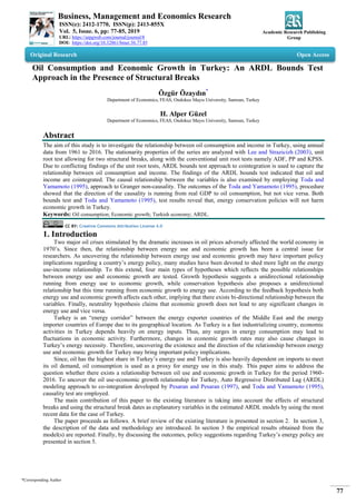
6. Business, Management and Economics Research
82
The coefficients of the variables and found to be positive and negative, respectively, which suggest
that a one unit change in the current year’s growth rate will cause a change in the oil consumption growth rate by
0.83 points in the same direction, while a change in the previous year’s growth rate will cause a 0.48 points change
in the current years oil consumption growth rate in the opposite direction.
The coefficient of the one period lagged error correction term (-0.15) is negative as expected and also
statistically significant, which suggests that 15% of the deviations from the long-run equilibrium level of oil
consumption will be corrected in the next period.
The ARDL (2,1) model is checked for normality with Jarque-Bera ( ) test, for serial correlation with Breusch-
Godfrey LM ( ) test, for heteroskedasticity with ARCH ( ) test and for model misspecification with Ramsey
RESET test. According to the results in Table 5 the model successfully passed all diagnostic tests. The
parameter stability of the model is also checked both with CUSUM and CUSUMSQ tests. The results of the
CUSUM and CUSUMSQ tests are presented in Figure.1.
Figure 1. CUSUM and CUSUMSQ Test Results
As can be seen from Figure 1 the estimated parameters of the ARDL (2,1) model are stable according to both
CUSUM and CUSUMSQ tests.
5.5. Toda-Yamamoto Causality Test
The causal relationship between the variables oil and real GDP is investigated by using Toda-Yamamoto
procedure. The results of the Toda-Yamamoto test based upon the Equation 9 and Equation 10 are presented in
Table 6.
Table-6. Toda-Yamamoto Causality Test Results
Null Hypothesis P-value Decision
3.58 0.05** Rejected
0.35 0.54 Not Rejected
Diagnostic Tests
3.12 (0.20) 14.74 (0.67)
a
The maximum lag length of the VAR Model is which suggested by AIC and
maximum order of integration is suggested by LS unit test. Thus, the
appropriate lag length of the VAR model is determined as ( .
b
There is no serial correlation or heteroskedasticity problem in the model.
* and ** denotes statistical significance at 1% and 5% level respectively.
According to the Toda-Yamamoto test results, the null hypothesis for equation 7 which suggests does not
cause is rejected. However, the null hypothesis for the equation 8 which suggests does not cause cannot
be rejected. Thus, the findings of the Toda and Yamamoto (1995), test revealed that there is a unidirectional
causality running from real GDP to oil consumption, but not vice versa.
6. Conclusion
In this study, the dynamic relationship between oil consumption and income for the case of Turkey is
investigated by using annual data over the period 1960-2016. Since the unit root test results were conflicting, ARDL
approach to cointegration is employed. Bounds test results confirmed that there exists a cointegrating relation
between oil consumption and economic growth, where economic growth found to be the long run forcing variable
for oil consumption. The findings of the long run parameters of the model revealed that a 1% increase in Real GDP

7. Business, Management and Economics Research
83
would lead to a 3.05% increase in oil consumption. The parameter estimates of the error correction model showed
that, 15% of the disequilibrium adjust back to the long run equilibrium within a year.
Apart from cointegration test, to uncover the direction of causality, Toda-Yamamoto version of Granger non-
causality test is also employed. The results of the Toda-Yamamoto test showed that there exists a unidirectional
causality running from economic growth to oil consumption which is consistent with the bounds test findings.
Both bounds test and Toda-Yamamoto test results suggested evidence in favor of the validity of conservation
hypothesis for the case of Turkey over the period 1960-2016, which implies energy conservation policies will not
harm economic growth in Turkey. Therefore, policy makers may take more brave steps to reduce the carbon
footprint of Turkey without concerning about economic growth.
.
References
Abosedra, S. and Baghestani, H. (1989). New evidence on the causal relationship between United States energy
consumption and gross national product. The Journal of Energy and Development, 14(2): 285-92.
Akarca, A. T. and Long, T. V. (1980). On the relationship between energy and GNP: a reexamination. The Journal
of Energy and Development, 5(2): 326-31.
Aktas, C. and Yilmaz, V. (2008). Causal relationship between oil consumption and economic growth in Turkey.
Kocaeli Üniversitesi Sosyal Bilimler Enstitüsü Dergisi, 15(1): 45-55.
Al-Mulali, U. (2011). Oil consumption, CO2 emission and economic growth in MENA countries. Energy,
36.10(2011): 6165-71.
Alam, M. S. and Paramati, S. R. (2015). Do oil consumption and economic growth intensify environmental
degradation? Evidence from developing economies. Applied Economics, 47(48): 5186-203.
Altinay, G. and Karagol, E. (2004). Structural break, unit root, and the causality between energy consumption and
GDP in Turkey. Energy Economics, 26(6): 985-94.
Altinay, G. and Karagol, E. (2005). Electricity consumption and economic growth: evidence from Turkey. Energy
Economics, 27(6): 849-56.
Aydin, M. (2018). The relationship between energy consumption and economic growth: the case of low- and middle-
income countries. Hacettepe Üniversitesi İktisadi ve İdari Bilimler Fakültesi Dergisi, 36(1): 1-15.
Behmiri, N. B. and Manso, J. R. P. (2013). How crude oil consumption impacts on economic growth of Sub-Saharan
Africa? Energy, 54(1): 74-83.
Bhusal, T. P. (2010). Econometric analysis of oil consumption and economic growth in Nepal. Economic Journal of
Development Issues, 11-12(1-2): 135-43.
Ceylan, R. and Başer, S. (2014). The analysis of the long-run relationship between oil consumption and real GDP in
Turkey through Johansen co-integration method. Business and Economics Research Journal, 5(2): 47-60.
Cheng, B. S. (1995). An investigation of cointegration and causality between energy consumption and economic
growth. The Journal of Energy and Development, 27(1): 73-84.
Cheng, B. S. and Lai, T. W. (1997). An investigation of co-integration and causality between energy consumption
and economic activity in Taiwan. Energy Economics, 19(4): 435-44.
Engle, R. F. and Granger, C. W. (1987). Co-integration and error correction: representation, estimation, and testing.
Econometrica: Journal of the Econometric Society, 55(2): 251-76.
Erol, U. and Yu, E. S. (1987). On the causal relationship between energy and income for industrialized countries.
The Journal of Energy and Development, 13(1): 113-22.
Ghali, K. H. and El-Sakka, M. I. (2004). Energy use and output growth in Canada: a multivariate cointegration
analysis. Energy Economics, 26(2): 225-38.
Ghosh, S. (2009). Import demand of crude oil and economic growth: Evidence from India. Energy Policy, 37(2):
699-702.
Glasure (2002). Energy and national income in Korea: further evidence on the role of omitted variables. Energy
Economics, 24(4): 355-65.
Glasure and Lee, A. R. (1997). Co-integration, error-correction, and the relationship between GDP and energy:the
case of South Korea and Singapore. Resource Energy Economics, 20(1): 17-25.
Gokmenoglu, K. and Taspinar, N. (2016). The relationship between CO2 emissions, energy consumption, economic
growth and FDI: the case of Turkey. The Journal of International Trade and Economic Development,
25(5): 706-23.
Granger (1969). Investigating causal relations by econometric models and cross-spectral methods. Econometrica:
Journal of the Econometric Society: 424-38.
Granger (1988). Some recent development in a concept of causality. Journal of Econometrics, 39(1-2): 199-211.
Gregory and Hansen, B. E. (1996a). Tests for cointegration in models with regime and trend Shifts. Oxford Bulletin
of Economics and Statistics, 58(3): 555–60.
Gregory and Hansen, B. (1996b). Residual-based Tests for cointegration in models with regime shifts. Journal of
Econometrics, 70: 99-126.
Hondroyiannis, G., Lolos, S. and Papapetrou, E. (2002). Energy consumption and economic growth: assessing the
evidence from Greece. Energy Economics, 24(4): 319-36.
Johansen, S. (1988). Statistical analysis of cointegration vectors. Journal of Economic Dynamics and Control, 12(2-
3): 231-54.
Johansen, S. and Juselius, K. (1990). Maximum likelihood estimation and inference on cointegration—with
applications to the demand for money. Oxford Bulletin of Economics and Statistics, 52(2): 169-210.

8. Business, Management and Economics Research
84
Karagöl, E., Erbaykal, E. and Ertuğrul, H. M. (2011). Economic growth and electricity consumption in Turkey: A
bound test approach. Doğuş Üniversitesi Dergisi, 8(1): 72-80.
Keskin, R. (2017). The relationship between economic growth and petroleum consumption in Turkey under
structural breaks. Yönetim ve Ekonomi: Celal Bayar Üniversitesi İktisadi ve İdari Bilimler Fakültesi
Dergisi, 24(3): 877-92.
Kraft, J. and Kraft, A. (1978). On the relationship between energy and GNP. The Journal of Energy and
Development, 3(2): 401-03.
Laurenceson, J. and Chai, J. C. (2003). Financial reform and economic development in China. Edward Elgar
Publishing.
Lee (2005). Energy consumption and GDP in developing countries: a cointegrated panel analysis. Energy
Economics, 27(3): 415-27.
Lee (2006). The causality relationship between energy consumption and GDP in G-11 countries revisited. Energy
Policy, 34(9): 1086-93.
Lee and Strazicizh, M. C. (2003). Minimum Lagrange Multiplier unit root test with two structural breaks. The
Review of Economics and Statistics, 85(4): 1082-89.
Lise, W. and Van Montfort, K. (2007). Energy consumption and GDP in Turkey: Is there a co‐integration
relationship? Energy Economics, 29(6): 1166-78.
Masih and Masih, R. (1996). Energy consumption, real income and temporal causality: results from a multi-country
study based on cointegration and error-correction modelling techniques. Energy Economics, 18(3): 165-83.
Masih and Masih, R. (1997). On the temporal causal relationship between energy consumption, real income, and
prices: some new evidence from Asian-energy dependent NICs based on a multivariate cointegration/vector
error-correction approach. Journal of Policy Modeling, 19(4): 417-40.
Mucuk, M. and Uysal, D. (2009). Energy consumption and economic growth in Turkish economy. Maliye Dergisi,
157(1): 105-15.
Narayan, P. K. (2005). The saving and investment nexus for China: evidence from cointegration tests. Applied
Economics, 37(17): 1979-90.
Oh, W. and Lee, K. (2004). Causal relationship between energy consumption and GDP revisited: the case of Korea
1970–1999. Energy Economics, 26(1): 51-59.
Ozata, E. (2010). Econometric investigation of the relationships between energy consumption and economic growth
in Turkey. Dumlupınar Üniversitesi Sosyal Bilimler Dergisi. 26.
Ozturk and Acaravci, A. (2010). CO2 emissions, energy consumption and economic growth in Turkey. Renewable
and Sustainable Energy Reviews, 14(9): 3220-25.
Ozturk and Acaravci, A. (2013). The long-run and causal analysis of energy, growth, openness and financial
development on carbon emissions in Turkey. Energy Economics, 36(1): 262-67.
Park, S. Y. and Yoo, S. H. (2014). The dynamics of oil consumption and economic growth in Malaysia. Energy
Policy, 66(1): 218-23.
Pesaran and Pesaran, B. (1997). Working with Microfit 4.0: An interactive econometric software package (DOS and
Windows versions). Oxford University Press: Oxford.
Pesaran and Smith, R. J. (1998). Structural analysis of cointegrating VARs. Journal of Economic Surveys, 12(1):
471–505.
Pesaran and Shin, Y. (1999). An autoregressive distributed lag modeling approach to cointegration analysis, in:
Strom, s., holly, a., diamond, p. (eds.), centennial volume of rangar frisch. Cambridge University Press:
Cambridge.
Pesaran and Pesaran, M. H. (2010). Time series econometrics using Microfit 5.0: A user's manual. Oxford
University Press, Inc.:
Pesaran, Shin, Y. and Smith, R. J. (2001). Bounds testing approaches to the analysis of level relationships. Journal
of Applied Econometrics, 16(3): 289–326.
Pinzón, K. (2018). Dynamics between energy consumption and economic growth in Ecuador: A granger causality
analysis. Economic Analysis and Policy, 57(1): 88-101.
Saatci, M. and Dumrul, Y. (2012). The relationship between energy consumption and economic growth: Evidence
from a structural break analysis for Turkey. International Journal of Energy Economics and Policy, 3(1):
20-29.
Saboori, B., Rasoulinezhad, E. and Sung, J. (2017). The nexus of oil consumption, CO2 emissions and economic
growth in China, Japan and South Korea. Environmental Science and Pollution Research, 24(8): 7436-55.
Soytas and Sari, R. (2003). Energy consumption and GDP: causality relationship in G-7 countries and emerging
markets. Energy Economics, 25(1): 33-37.
Soytas and Sari, R. (2006). Energy consumption and income in G-7 countries. Journal of Policy Modeling, 28(7):
739-50.
Soytas and Sari, R. (2009). Energy consumption, economic growth, and carbon emissions: challenges faced by an
EU candidate member. Ecological Economics, 68(6): 1667-75.
Soytas, Sari, R. and Ozdemir, O. (2001). Energy consumption and GDP relation in Turkey: a cointegration and
vector error correction analysis. Economies and Business in Transition: Facilitating Competitiveness and
Change in The Global Environment Proceedings, 1: 838-44.
Stern, D. I. (2000). A multivariate cointegration analysis of the role of energy in the US macroeconomy. Energy
Economics, 22(2): 267-83.

9. Business, Management and Economics Research
85
Toda, H. Y. and Yamamoto, T. (1995). Statistical inference in vector autoregressions with possibly integrated
processes. Journal of Econometrics, 66(1-2): 225-50.
Ucak, S. and Usupbeyli, A. (2015). The causality relationship between oil consumption and economic growth in
Turkey. Ankara Üniversitesi SBF Dergisi, 70(3): 769-87.
Wang, S., Li, Q., Fang, C. and Zhou, C. (2016). The relationship between economic growth, energy consumption,
and CO2 emissions: Empirical evidence from China. Science of the Total Environment, 542(A): 360-71.
Yazdan, G. F. and Hossein, S. S. M. (2012). Causality between oil consumption and economic growth in Iran: An
ARDL testing approach. Asian Economic and Financial Review, 2(6): 678-86.
Yu and Hwang, B. K. (1984). The relationship between energy and GNP: further results. Energy Economics, 6(3):
186-90.
Yu and Choi, J. Y. (1985). The causal relationship between energy and GNP: an international comparison. The
Journal of Energy and Development, 10(2): 249-72.
Yuan, Zhao, C., Yu, S. and Hu, Z. (2007). Electricity consumption and economic growth in China: cointegration and
co-feature analysis. Energy Economics, 26(6): 1179-91.
Yuan, Kang, J. G., Zhao, C. H. and Hu, Z. G. (2008). Energy consumption and economic growth: evidence from
China at both aggregated and disaggregated levels. Energy Economics, 30(6): 3077-94.
Zamani, M. (2007). Energy consumption and economic activities in Iran. Energy Economics, 29(6): 1135-40.