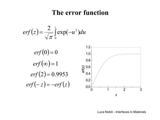
Download as PDF, PPTX
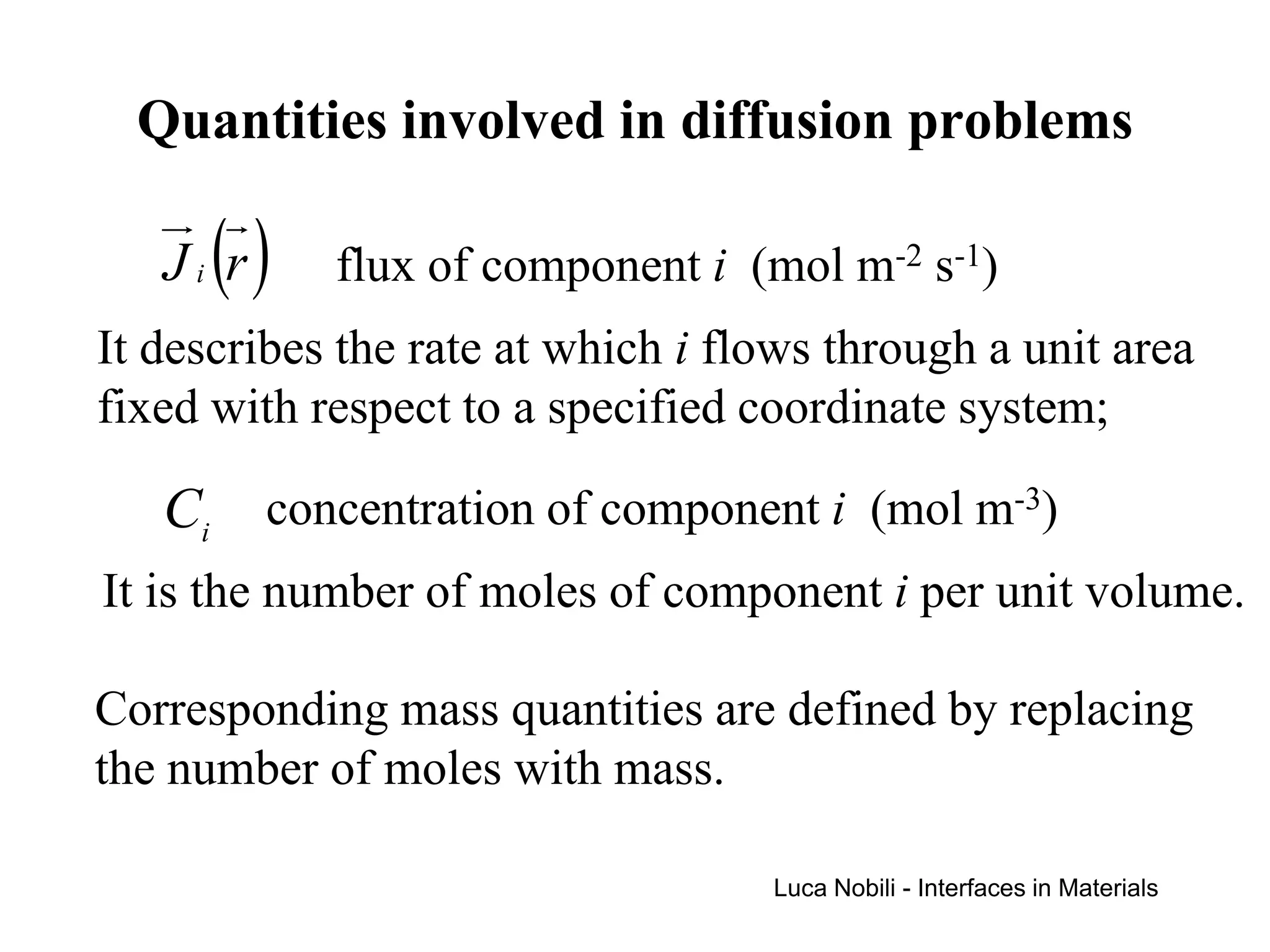
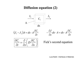
![Thermodynamic factor (2)
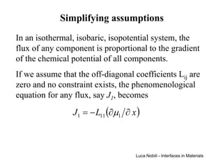
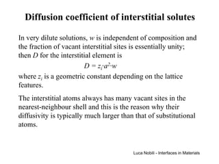
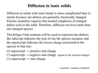
It may be assumed that the total concentration of a
solid system is constant; then Ci depends only on ni:
Ci = niC
The expressions of Ji become
M i Ci RT [∂ ln (ni ) ∂x + ∂ ln (γ i ) ∂x ] = Di C ∂ni ∂x
∂x
Di = M i RTni [∂ ln(ni ) ∂x + ∂ ln(γ i ) ∂x]
∂ni
Di = M i RT [1 + ∂ ln (γ i ) ∂ ln (ni )]
Luca Nobili - Interfaces in Materials](https://image.slidesharecdn.com/pdiffusion1-120311210306-phpapp02/85/P-diffusion_1-12-320.jpg)
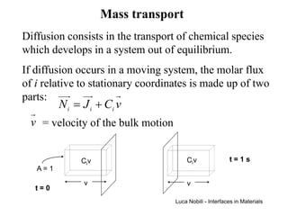
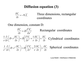
![Relationship between Di and *Di
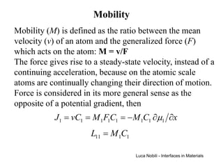
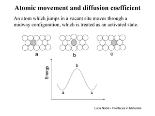
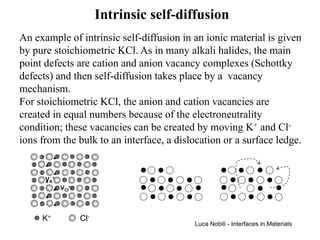
In a binary diffusion couple with no concentration
gradient, the self-diffusion coefficient (*Di) is given by:
*
Di =*M i RT [1 + ∂ ln ( *γ i ) ∂ ln ( * ni )]
Since the stable and radioactive isotopes are chemically
identical, γi will be independent on the *ni/ni ratio and
will be constant, then
*
Di =*M i RT
If it is assumed that *Mi = Mi, a relationship is obtained
between intrinsic diffusivity and self-diffusivity:
Di =*Di [1 + ∂ ln (γ i ) ∂ ln (ni )]
Luca Nobili - Interfaces in Materials](https://image.slidesharecdn.com/pdiffusion1-120311210306-phpapp02/85/P-diffusion_1-14-320.jpg)
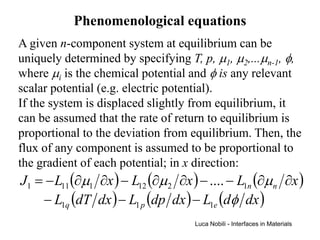
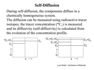
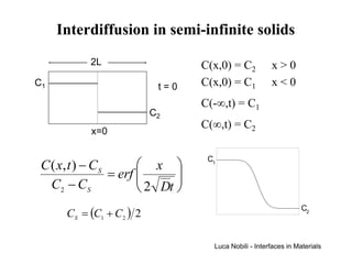
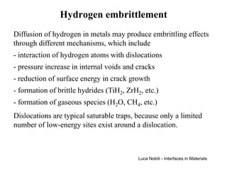
![Interdiffusion experiments (3)
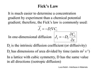
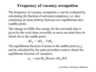
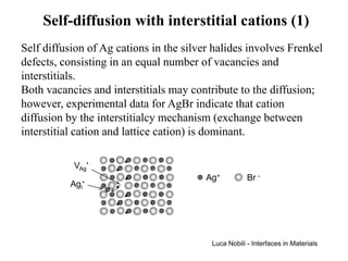
The flux relative to specimen ends can be expressed according
to the Fick’ law by defining the interdiffusion coefficient
D = D1 ⋅ n2 + D2 ⋅ n1
Consequently, the concentration profile is obtained by solving
the diffusion equation
∂Ci ∂ 2 Ci
=D 2
∂t ∂x
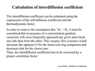
The interdiffusion coefficient can be expressed in term of the
self-diffusion coefficients:
D = ( * D1n2 + *D2 n1 )[1 + ∂ ln (γ 1 ) ∂ ln (n1 )]
From the Gibbs-Duhem equation, ∂ ln (γ 1 ) ∂ ln (n1 ) = ∂ ln (γ 2 ) ∂ ln (n2 )
Luca Nobili - Interfaces in Materials](https://image.slidesharecdn.com/pdiffusion1-120311210306-phpapp02/85/P-diffusion_1-18-320.jpg)
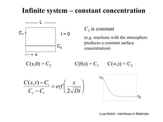
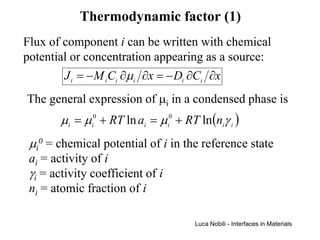
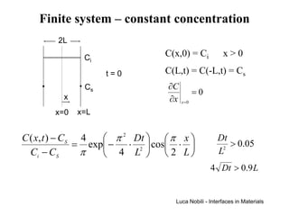
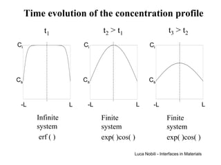
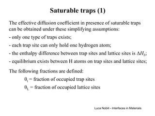
![Solution for infinite systems
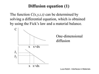
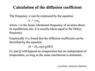
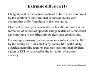
C1
C ( x, t ) − C1 x
= erf
C2 − C1 2 Dt C2
x = 4 Dt
Each value of the ratio (C-C1)/(C2-C1) is associated with a
particular value of z = x/[2(Dt)1/2];
each composition moves away from the plane of x = 0 at a rate
proportional to (Dt)1/2 (except C = C1 which remains at x = 0).
The system can be treated as infinite if the diffusion distance is
small relative to the length of the system (L):
2 Dt << L (4 Dt < L )
Luca Nobili - Interfaces in Materials](https://image.slidesharecdn.com/pdiffusion1-120311210306-phpapp02/85/P-diffusion_1-24-320.jpg)
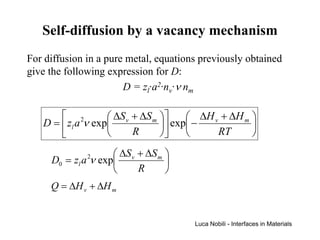

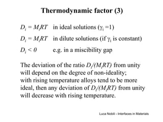
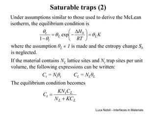
![Self-diffusion in dilute alloys
In a binary substitutional solution, there are relationships
between self-diffusion coefficients of components 1 and 2.
It has been observed that if D1 decreases with the atomic
fraction of solute 2 (n2), then D2 also decreases with n2. These
relationships are often expressed by the equations:
D1(n2) = D1(0)[1+b1n2] D2(n2) = D2(0)[1+B1n2]
thus b1 and B1 have the same sign.
The effect of the solute can be thought to be the addition of
regions of a different jump frequency (a higher frequency if b is
positive), probably because the effect of the solute is to modify
the vacancy concentration.
Luca Nobili - Interfaces in Materials](https://image.slidesharecdn.com/pdiffusion1-120311210306-phpapp02/85/P-diffusion_1-45-320.jpg)
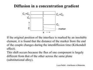
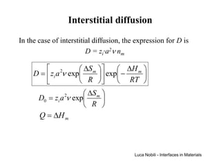
![Self-diffusivity in alkali halides (1)
The defect creation can be written as a reaction:
null = VK' + VCl
•
The equilibrium constant of this reaction (Keq) is related to
the molar free energy of formation (∆GS) of the Schottky
pair; for small concentrations of the vacancies, activities can
be taken equal to the site fractions:
[V ]⋅ [V ] = K
K
' •
Cl eq
= exp(− ∆GS RT )
the square brackets indicate a site fraction.
Luca Nobili - Interfaces in Materials](https://image.slidesharecdn.com/pdiffusion1-120311210306-phpapp02/85/P-diffusion_1-60-320.jpg)
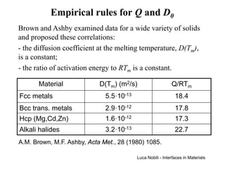
![Self-diffusivity in alkali halides (2)
Electrical neutrality requires that [VK' ] = [VCl ]
•
Then [V ] = [V ] = exp(− ∆G
K
' •
Cl S
2 RT )
The self-diffusivity of K is given by:
*
DK = zl a 2 fν exp[(∆S S 2 + ∆S m ) R ]exp[− (∆H S 2 + ∆H m ) RT ]
CV CV
The activation energy for self-diffusion is then
Q = ∆H S 2 + ∆H m CV
A similar expression applies to Cl self-diffusion on the
anion sublattice.
Luca Nobili - Interfaces in Materials](https://image.slidesharecdn.com/pdiffusion1-120311210306-phpapp02/85/P-diffusion_1-61-320.jpg)
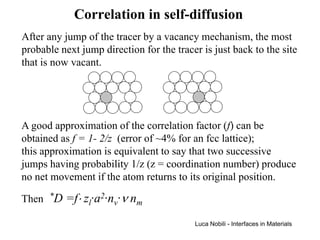
![Self-diffusion with interstitial cations (2)
The reaction of formation of cation Frenkel pairs is:
Ag × = Ag i• + VAg
Ag
'
The activity of the lattice cation is unity, then
[Ag ]⋅ [V ] = K
•
i
'
Ag eq = exp(− ∆GF RT )
The electrical neutrality requires that fractions of vacancies
and interstitials are equal:
[Ag ] = [V ] = exp[− (∆G 2) RT ]
•
i
'
Ag F
The activation energy for self-diffusivity of the Ag cations is
Q = ∆H F 2 + ∆H m
I
Luca Nobili - Interfaces in Materials](https://image.slidesharecdn.com/pdiffusion1-120311210306-phpapp02/85/P-diffusion_1-63-320.jpg)
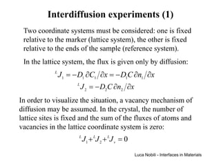
![Extrinsic diffusion (2)
Fractions of anionic and cationic vacancies are related to
the content of the extrinsic Ca++ impurity:
[Ca ]+ [V ] = [V ]
•
K
•
Cl
'
K
By inserting this relationship in the expression of the
equilibrium constant, the following equation is obtained:
[V ]⋅ ([V ]− [Ca ]) = exp(− ∆G
'
K
'
K
•
K S RT ) = V [ ]' 2
K pure
Solution to this equation is
[Ca ]
[ ]
12
4 VK pure
' 2
[V ] = 2
•
' K 1 + 1 +
K
[ ] • 2
Ca K
Luca Nobili - Interfaces in Materials](https://image.slidesharecdn.com/pdiffusion1-120311210306-phpapp02/85/P-diffusion_1-65-320.jpg)
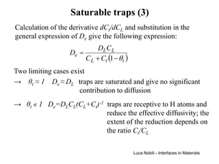
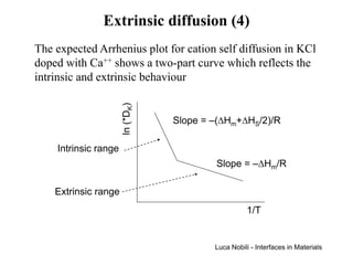
![Extrinsic diffusion (3)
There are two limiting cases for the behaviour of the cation
vacancy fraction:
Intrinsic [V ]
'
K pure [ ]•
>> Ca K [V ] = [V ]
'
K
'
K pure
Extrinsic [V ]
'
K pure << [Ca ]
•
K
[V ] = [Ca ]
'
K
•
K
The intrinsic case applies at small doping levels or at high
temperatures; the activation energy for cation self-diffusion is
the same as in the pure material.
The extrinsic case applies at large doping levels or at low
temperatures; the fraction of cation vacancies is equal to the
impurity fraction and is therefore temperature independent;
the activation energy consists only of the migration term.
Luca Nobili - Interfaces in Materials](https://image.slidesharecdn.com/pdiffusion1-120311210306-phpapp02/85/P-diffusion_1-66-320.jpg)
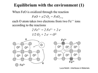
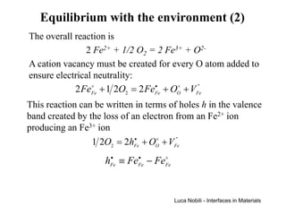
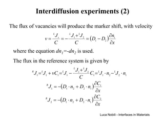
![Equilibrium with the environment (3)
Reaction 1 2O2 = 2hFe + OO + VFe
• × ''
Equilibrium [V ]⋅ [h ] = K
'' • 2
= exp(− ∆G RT )
(p )
Fe Fe
Constant 12 eq
O2
Neutrality
condition
[h ] = 2[V ]
•
Fe
''
Fe
The equilibrium fraction of cation vacancies is
13
[VFe'' ] = 1 ( pO )1 6 exp[− ∆G (3RT )]
4 2
The cation self-diffusivity due to the vacancy mechanism
varies as the one-sixth power of the oxygen partial pressure
Luca Nobili - Interfaces in Materials](https://image.slidesharecdn.com/pdiffusion1-120311210306-phpapp02/85/P-diffusion_1-71-320.jpg)


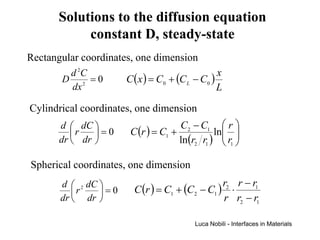
1) The document describes various quantities and concepts related to diffusion, including molar flux, concentration, mass transport, phenomenological equations, mobility, and Fick's laws. 2) It discusses diffusion in different coordinate systems and provides the diffusion equation for one-dimensional diffusion in rectangular, cylindrical, and spherical coordinates. 3) Solutions to the diffusion equation are presented for both steady-state and non-steady-state diffusion in various systems, including using error functions for an infinite system.


![PM [D01] Matter Waves](https://cdn.slidesharecdn.com/ss_thumbnails/pmd01matterwaves-151027082009-lva1-app6892-thumbnail.jpg?width=640&height=640&fit=bounds)


![lecture 5 PHASE TRANSFORMATIONS in Metal and Alloys [Autosaved].pptx](https://cdn.slidesharecdn.com/ss_thumbnails/lecture5phasetransformationsinmetalandalloysautosaved-250304103627-a1a7e4b4-thumbnail.jpg?width=640&height=640&fit=bounds)


