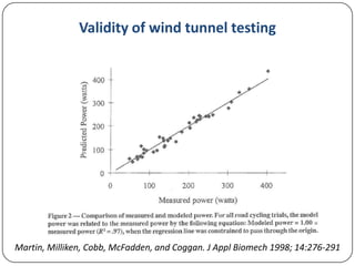
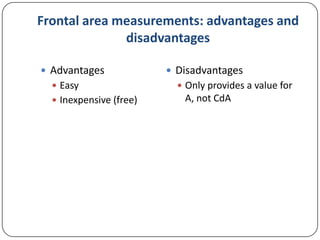
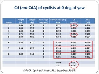
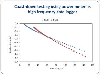
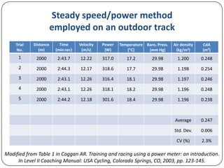
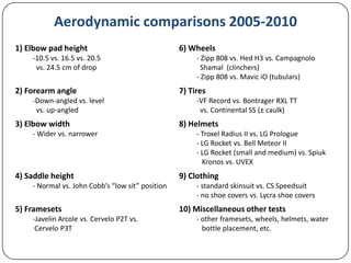
Aerodynamic testing without a wind
tunnel: from the simple to the sublime
Andrew R. Coggan, Ph.D.
Outline of talk

 Wind tunnel testing/the physics of cycling
 Alternatives to wind tunnel testing
Wind tunnel testing: how do you do it?
Wind tunnel testing:
advantages and disadvantages
 Advantages
 Accuracy
 Precision/sensitivity
 Speed
 Ability to test at multiple

yaw angles

 Disadvantages
 Cost!
CdA as a function of yaw angle
0.250

CdA (m2)

0.200
0.150
Std aero position
Superman position

0.100
0.050
0.000
0

5

10

Yaw angle (deg)

15
Validity of wind tunnel testing

Martin, Milliken, Cobb, McFadden, and Coggan. J Appl Biomech 1998; 14:276-291
Mathematical model of the physics of cycling
PTOT = (PAT + PKE + PRR + PWB + PPE)/Ec
PTOT = (0.5ρVa2Vg(CdA + Fw) + 0.5(mt + I/r2)(Vgf2 - Vgi2)/(tf - ti) + VgCrrmtgCOS(TAN-1(Gr)) +
Vg(0.091+0.0087Vg) + VgmtgSIN(TAN-1(Gr)))/Ec
Where:
PTOT = total power required (W)
PAT = power required to overcome total aerodynamic drag (W)
PKE = power required to change kinetic energy (W)
PRR = power required to overcome rolling resistance (W)
PWB = power required to overcome drag of wheel bearings (W)
PPE = power required to change potential energy (W)
ρ = air density (kg/m3)
Va = air velocity (relative to direction of travel) (m/s)
Vg = ground velocity (m/s)
Cd = coefficient of drag (dependent on wind direction) (unitless)
A = frontal area of bike+rider system (m2)
FW = wheel rotation factor (expressed as incremental frontal area) (m2)

mt= total mass of bike+rider system (kg)
I = moment of inertia of wheels (kgm2)
r = outside radius of tire (m)
Vgf = final ground velocity (m/s)
Vgi = initial ground velocity (m/s)
tf = final time (s)
ti = initial (s)
Crr = coefficient of rolling resistance (unitless)
g = acceleration due to gravity (9.81 m/s2)
Gr = road gradient (unitless)
Ec = efficiency of chain drive system (unitless)

Martin, Milliken, Cobb, McFadden, and Coggan. J Appl Biomech 1998; 14:276-291
Alternatives to wind tunnel testing
 Methods not requiring a power meter
 Frontal area measurements from photographs
 Coast-down testing
 Methods requiring a power meter
 Steady speed/power
 “Classical” regression method
 Robert Chung’s virtual elevation method
 Adam Haile’s short track regression method
Measuring frontal area: how do you do it?

Kyle CR. Cycling Science 1991; Sept/Dec: 51-56.
Frontal area measurements: advantages and
disadvantages
 Advantages
 Easy
 Inexpensive (free)

 Disadvantages
 Only provides a value for

A, not CdA
Cd (not CdA) of cyclists at 0 deg of yaw

Subject
1
2
3
4
5

Height
(m)
1.63
1.80
1.80
1.75
1.80

Weight
(kg)
47.6
77.0
74.0
59.9
69.0

Yaw angle
(degrees)
0
0
0
0
0

Frontal area (m2)
Total
0.272
0.279
0.290
0.334
0.358

Cd
(unitless)
0.793
0.718
0.680
0.652
0.655

CdA
(m2)
0.216
0.200
0.197
0.218
0.234

6

1.86

81.0

7

1.93

87.0

8

1.80

74.0

0
0
0
0
0
0

0.284
0.264
0.310
0.280
0.310
0.285

0.705
0.719
0.712
0.763
0.703
0.672

0.200
0.190
0.221
0.214
0.218
0.192

Mean
S.D.

0.707
0.043

Kyle CR. Cycling Science 1991; Sept/Dec: 51-56.
Relationship of CdA to frontal area
0.250

0.200
y = 0.380x + 0.096
R² = 0.595

CdA (m2)

0.150

0.100

0.050

0.000
0.000

0.100

0.200
Frontal area (m2)

0.300

Kyle CR. Cycling Science 1991; Sept/Dec: 51-56.

0.400
Cd of model rockets

DeMar JS. National Asssociation of Rocketry Report NAR52094, July 1995.
Coast-down testing: how do you do it?
Method 1: coast down a long, steady hill and
record either time or maximal speed.
Method 2: coast down from a higher to a lower
speed on a constant (flat) grade and record rate of
decelleration.
Coast-down testing
 Advantages
 Can be inexpensive

(free)

 Disadvantages
 Requires idealized

venue and weather
conditions
 Can be difficult to
achieve high precision
 Time-consuming
Coast-down testing: indoors

CV across 4 trials for CdA: 0.56% (n = 30 per trial)
CV across 4 trials for Crr: 0.59% (n = 30 per trial)

CV across 4 trials for CdA: 1.16% (n = 15 per trial)
CV across 4 trials for Crr: 1.83% (n = 15 per trial)

Candau et al. Med Sci Sports Exerc 1999; 31:1441-1447.
Coast-down testing: outdoors

CV across 12 trials for CdA: 9.2%
CV across 12 trials for Crr: 138%

Cameron. Human Power 1995; 12:7-11
Coast-down testing using power meter as
high frequency data logger
Trial 1

Trial 2

14
12

Speed (m/s)

10
8
6
4
2
0
0

10

20

30
Time (s)

40

50

60
Coast-down testing using power meter as
high frequency data logger
Trial 1

Trial 2

60

80

0.0
-0.2

Acceleration (m/s2)

-0.4
-0.6
-0.8

-1.0
-1.2
-1.4
-1.6
-1.8
-2.0
0

20

40

Speed2 (m2/s2)

100

120

140

160
Steady speed/power method:
how do you do it?
Ride at a steady speed (or power) on a constant
(flat) grade while recording average power (or
average speed).
Steady speed/power method
 Advantages
 Data analysis is simple

 Disadvantages
 Requires idealized

venue and weather
conditions
 Does not differentiate
between Crr and CdA
Steady speed/power method
employed on an outdoor track
Trial
No.

Distance
(m)

Time
(min:sec)

Velocity
(m/s)

Power
(W)

1

2000

2:43.7

12.22

317.0

17.2

2

2000

2:44.3

12.17

318.6

3

2000

2:43.1

12.26

4

2000

2:43.1

5

2000

2:44.2

Temperature Baro. Press.
(mm Hg)
(C)

Air density
(kg/m3)

CdA
(m2)

29.98

1.200

0.248

17.7

29.98

1.198

0.254

316.4

18.1

29.98

1.197

0.246

12.26

318.1

18.2

29.98

1.196

0.248

12.18

301.6

18.4

29.98

1.196

0.238

Average

0.247

Std. Dev.

0.006

CV (%)

2.3%

Modified from Table 1 in Coggan AR. Training and racing using a power meter: an introduction.
In Level II Coaching Manual: USA Cycling, Colorado Springs, CO, 2003, pp. 123-145.
“Classical” regression method:
how do you do it?
Ride at a range of steady speeds on a constant (flat)
grade while recording average power (and speed).
“Classical” regression method
 Advantages

 Disadvantages

 High accuracy and

 Time-consuming

precision attainable
 Differentiates between
CdA and Crr (mu)

 Requires idealized

venue and weather
conditions
Accuracy of the regression approach
Subject

Wind tunnel
CdA (m2)

Field test
CdA (m2)

Difference
(m2)

Difference
(%)

1

0.247

0.252

+0.005

+2.0%

2

0.291

0.269

-0.022

-7.6%

3

0.240

0.241

+0.001

+0.4%

4

0.251

0.251

0.000

0.0%

5

0.252

0.253

+0.001

+0.4%

6

0.285

0.283

-0.002

-0.7%

7

0.198

0.198

0.000

0.0%

Mean

0.252

0.250

-0.002

-0.8%

S.D.

0.031

0.027

0.009

3.1%

Data for subjects 1-6 are from Martin JC et al. Med Sci Sports Exerc 2006; 38:592-597,
whereas data for subject 7 are unpublished observations of the presenter.
Taking the Tom Compton challenge:
the experiment
Taking the Tom Compton challenge: results
Expected

Measured

Difference in aerodynamic drag (N)

0.35
0.30
0.25
0.20
0.15
0.10

0.05
0.00
6.4 cm sphere

10.2 cm sphere
Determination of Crr via regression testing
Crr from Andy's field tests (regression method)

0.0060

y = 1.087x + 0.000
R² = 0.949

Y=X

0.0050
0.0040
0.0030

Continental SS (clinchers)

Continental SS + Bontrager RXL
TT (clinchers)
VF Record (clinchers)
Bontrager RXL TT (clinchers)

Bad cassette
bearings!

0.0020
0.0010
0.0000
0.000 0.001 0.002 0.003 0.004 0.005 0.006
Crr from Al's roller testing

VF Record + Tufo S3 Pro
(tubulars)
Michelin Pro Race 2 SC
(clinchers)
VF Record (tubular) + Vred
Fortezza Tricomp (clincher)
Continental Ultra 2000
(clinchers)
Bontrager RXL TT (clinchers)
Aerodynamic comparisons 2005-2010
1) Elbow pad height
-10.5 vs. 16.5 vs. 20.5
vs. 24.5 cm of drop

2) Forearm angle
-Down-angled vs. level
vs. up-angled

3) Elbow width
- Wider vs. narrower

4) Saddle height
- Normal vs. John Cobb’s “low sit” position

5) Framesets
-Javelin Arcole vs. Cervelo P2T vs.
Cervelo P3T

6) Wheels
- Zipp 808 vs. Hed H3 vs. Campagnolo
Shamal (clinchers)
- Zipp 808 vs. Mavic iO (tubulars)

7) Tires
-VF Record vs. Bontrager RXL TT
vs. Continental SS (± caulk)

8) Helmets
- Troxel Radius II vs. LG Prologue
- LG Rocket vs. Bell Meteor II
- LG Rocket (small and medium) vs. Spiuk
Kronos vs. UVEX

9) Clothing
- standard skinsuit vs. CS Speedsuit
- no shoe covers vs. Lycra shoe covers

10) Miscellaneous other tests
- other framesets, wheels, helmets, water
bottle placement, etc.
Centaur Road in Chesterfield, MO

The Centaur Road
“natural wind
tunnel”
Centaur Road: a “natural wind tunnel”

Photo courtesy of Mark Ewers
Temperature data from 11/2/2008
25
Brunton
removed
from car and
hung on sign

Temperature (deg C)

20

15

Brunton removed
from sign and
placed in skinsuit

Period of data
collection

10

5

Sun reaches
into woods

0
6:45:00

7:15:00

7:45:00

8:15:00

Time

8:45:00

9:15:00
Beware of local variations
in environmental conditions!

Airport temperature (deg C)

30
25

y = 1.151x - 0.711
R² = 0.952

20
15
10
5
0
0

5

10
15
20
Brunton temperature (deg C)

25

30
CdA and Crr determined using the regression
method (non-linear fit)
West

East

450
400
y = 0.1339x2 + 2.924
R² = 0.9989

350
Power (W)

300
250
200
150

CdA = 0.233 ± 0.004 m2
Crr = 0.00387 ± 0.00039

100
50
0
0

2

4

6

8
Speed (m/s)

10

12

14

16
CdA and Crr determined using the regression
method (linear fit)
West

East

30
25

y = 0.134x + 2.889
R² = 0.997

Force (N)

20
15
CdA = 0.233 ± 0.003 m2
Crr = 0.00382 ± 0.00029

10
5
0
0

25

50

75

100
Speed2 (m2/s2)

125

150

175

200
CdA and Crr determined using the regression
method (worst case scenario)
East

West

30
y = 0.135x + 4.064
R² = 0.941

25

Force (N)

20
15
CdA = 0.232 ± 0.017 m2
Crr = 0.00515 ± 0.00135

10

5
0
0

25

50

75

100
Speed2 (m2/s2)

125

150

175

200
CdA and Crr determined using the regression
method (assuming constant wind)
East

West

30
y = 0.1356x + 4.000
R² = 0.9975

25

Force (N)

20
15

CdA = 0.233 ± 0.003 m2
Crr = 0.00506 ± 0.00027
Est. wind = 0.49 m/s

10

5
0
0

25

50

75

100
Speed2 (m2/s2)

125

150

175

200
Using a power meter as a wind meter
0.5
0.4
y = 0.646x - 0.0331
R² = 0.413
P<0.05

Relative apparent wind speed
from regression (m/s)

0.3
0.2
0.1
0

Average wind speeds (m/s)
iBike: -0.06 ± 0.18
Regr: -0.06 ± 0.18

-0.1
-0.2
-0.3

-0.4
-0.5
-0.5

-0.4

-0.3

-0.2

-0.1

0

0.1

0.2

Relative wind speed from iBike (m/s)

0.3

0.4

0.5
The Beaufort scale
Wind is thine enemy!!
Robert Chung’s “virtual elevation” (VE)
method: how do you do it?
The VE method is really more of a post-hoc analytical
approach than it is a formal means of performing field tests.
Typically, however, it applied to data collected while riding
out-and-back along the same stretch of road or around and
around the same loop, while allowing speed and power to vary.
Changes in kinetic and potential energy are then taken into
consideration in the calculations, leveraging the knowledge
that the same point on the road is always at the same elevation
to calculate a “virtual elevation” that reflects the true elevation
plus any unexplained variability due to, e.g., wind.
Robert Chung’s VE method
 Advantages

 Disadvantages

 Allows use of wider

 Data dropouts can be a

variety of venues
 Often faster than
regression testing
 High precision attainable

PITA
 Can often be difficult to
differentiate between Δ in
CdA and Δ in Crr (mu)
 Accuracy?
 Does not account for wind
City Hall Drive in Ballwin, MO
Speed, power, and virtual elevation during a
representative lap of City Hall Drive
Speed (m/s)

Virtual elevation (m)

Power (W)
500

10

400

5
300
0
200
-5
100

-10
-15

0
3.15

3.35

3.55
Distance (km)

3.75

3.95

Power (W)

Speed (m/s) or virtual Elevation (m)

15
VE profile of 8 laps of City Hall Drive
Crr: 0.0038 (assumed)

CdA: 0.305 m2

15

Virtual Elevation (m)

10
1

2

4

3

5

5

6

7

8

0
-5

-10
-15

0

1

2

3

4

Distance (km)

5

6

7
VE profile of 8 laps of City Hall Drive
Crr: 0.0057 (assumed)

CdA: 0.280 m2

15

Virtual Elevation (m)

10
1

2

5

4

3

5

6

7

8

0

-5
-10
-15
0

1

2

3

4

Distance (km)

5

6

7
VE profile of 8 laps of City Hall Drive
Crr: 0.0019 (assumed)

CdA: 0.331 m2

15

Virtual Elevation (m)

10
1

2

5

4

3

5

6

7

8

0
-5
-10
-15
0

1

2

3

4

Distance (km)

5

6

7
Effect of wind on CdA estimated using
the VE approach
150

2007
Actual CdA: 0.208 m2
Apparent CdA: 0.237 m2
Chung CdA: 0.242 m2

100

Virtual Elevation (m)

50
0

2004
Actual CdA: 0.228 m2
Apparent CdA: 0.234 m2
Chung CdA: 0.248 m2

-50
-100

2008
Actual CdA: 0.225 m2
Apparent CdA: 0.238 m2
Chung CdA: 0.231 m2

-150

-200
-250
0

5

10
Distance from start (km)

15

20
Wind is thine enemy!!
Adam Haile’s short track regression method:
method: how do you do it?
Similar to the classical regression approach, Crr and CdA are
derived by regressing force on velocity. However, rather than
utilizing average values obtained during each “run”, the short
track regression method uses each lap-length segment of data
extractable from multiple short laps. Since each lap starts and
ends in the same place (at least theoretically), variations in
potential energy can be ignored. On the other hand, speed is
allowed to vary within laps (and must vary across laps), with
variations in kinetic energy accounted for in the calculations
Adam Haile’s
short track regression method
 Advantages

 Disadvantages

 High precision

 Data dropouts can be a

attainable
 Differentiates between
CdA and Crr (mu)
 Allows use of wider
variety of venues
 Faster than regression
testing (?)

PITA
 Accuracy?
 Does not account for
wind
Example data from short track regression
testing on an indoor track
Summary and conclusions
 A wide variety of methods exist for estimating CdA

without use of a wind tunnel. Each has its advantages
and disadvantages, with the quality of the data
depending more upon attention to detail and
access/selection of an appropriate test venue than
upon the exact method used. The best choice will
therefore depend upon an individual’s specific
circumstances.

Aero testing without a wind tunnel

  • 1.
    Aerodynamic testing withouta wind tunnel: from the simple to the sublime Andrew R. Coggan, Ph.D.
  • 2.
    Outline of talk Wind tunnel testing/the physics of cycling  Alternatives to wind tunnel testing
  • 3.
    Wind tunnel testing:how do you do it?
  • 4.
    Wind tunnel testing: advantagesand disadvantages  Advantages  Accuracy  Precision/sensitivity  Speed  Ability to test at multiple yaw angles  Disadvantages  Cost!
  • 5.
    CdA as afunction of yaw angle 0.250 CdA (m2) 0.200 0.150 Std aero position Superman position 0.100 0.050 0.000 0 5 10 Yaw angle (deg) 15
  • 6.
    Validity of windtunnel testing Martin, Milliken, Cobb, McFadden, and Coggan. J Appl Biomech 1998; 14:276-291
  • 7.
    Mathematical model ofthe physics of cycling PTOT = (PAT + PKE + PRR + PWB + PPE)/Ec PTOT = (0.5ρVa2Vg(CdA + Fw) + 0.5(mt + I/r2)(Vgf2 - Vgi2)/(tf - ti) + VgCrrmtgCOS(TAN-1(Gr)) + Vg(0.091+0.0087Vg) + VgmtgSIN(TAN-1(Gr)))/Ec Where: PTOT = total power required (W) PAT = power required to overcome total aerodynamic drag (W) PKE = power required to change kinetic energy (W) PRR = power required to overcome rolling resistance (W) PWB = power required to overcome drag of wheel bearings (W) PPE = power required to change potential energy (W) ρ = air density (kg/m3) Va = air velocity (relative to direction of travel) (m/s) Vg = ground velocity (m/s) Cd = coefficient of drag (dependent on wind direction) (unitless) A = frontal area of bike+rider system (m2) FW = wheel rotation factor (expressed as incremental frontal area) (m2) mt= total mass of bike+rider system (kg) I = moment of inertia of wheels (kgm2) r = outside radius of tire (m) Vgf = final ground velocity (m/s) Vgi = initial ground velocity (m/s) tf = final time (s) ti = initial (s) Crr = coefficient of rolling resistance (unitless) g = acceleration due to gravity (9.81 m/s2) Gr = road gradient (unitless) Ec = efficiency of chain drive system (unitless) Martin, Milliken, Cobb, McFadden, and Coggan. J Appl Biomech 1998; 14:276-291
  • 8.
    Alternatives to windtunnel testing  Methods not requiring a power meter  Frontal area measurements from photographs  Coast-down testing  Methods requiring a power meter  Steady speed/power  “Classical” regression method  Robert Chung’s virtual elevation method  Adam Haile’s short track regression method
  • 9.
    Measuring frontal area:how do you do it? Kyle CR. Cycling Science 1991; Sept/Dec: 51-56.
  • 10.
    Frontal area measurements:advantages and disadvantages  Advantages  Easy  Inexpensive (free)  Disadvantages  Only provides a value for A, not CdA
  • 11.
    Cd (not CdA)of cyclists at 0 deg of yaw Subject 1 2 3 4 5 Height (m) 1.63 1.80 1.80 1.75 1.80 Weight (kg) 47.6 77.0 74.0 59.9 69.0 Yaw angle (degrees) 0 0 0 0 0 Frontal area (m2) Total 0.272 0.279 0.290 0.334 0.358 Cd (unitless) 0.793 0.718 0.680 0.652 0.655 CdA (m2) 0.216 0.200 0.197 0.218 0.234 6 1.86 81.0 7 1.93 87.0 8 1.80 74.0 0 0 0 0 0 0 0.284 0.264 0.310 0.280 0.310 0.285 0.705 0.719 0.712 0.763 0.703 0.672 0.200 0.190 0.221 0.214 0.218 0.192 Mean S.D. 0.707 0.043 Kyle CR. Cycling Science 1991; Sept/Dec: 51-56.
  • 12.
    Relationship of CdAto frontal area 0.250 0.200 y = 0.380x + 0.096 R² = 0.595 CdA (m2) 0.150 0.100 0.050 0.000 0.000 0.100 0.200 Frontal area (m2) 0.300 Kyle CR. Cycling Science 1991; Sept/Dec: 51-56. 0.400
  • 13.
    Cd of modelrockets DeMar JS. National Asssociation of Rocketry Report NAR52094, July 1995.
  • 14.
    Coast-down testing: howdo you do it? Method 1: coast down a long, steady hill and record either time or maximal speed. Method 2: coast down from a higher to a lower speed on a constant (flat) grade and record rate of decelleration.
  • 15.
    Coast-down testing  Advantages Can be inexpensive (free)  Disadvantages  Requires idealized venue and weather conditions  Can be difficult to achieve high precision  Time-consuming
  • 16.
    Coast-down testing: indoors CVacross 4 trials for CdA: 0.56% (n = 30 per trial) CV across 4 trials for Crr: 0.59% (n = 30 per trial) CV across 4 trials for CdA: 1.16% (n = 15 per trial) CV across 4 trials for Crr: 1.83% (n = 15 per trial) Candau et al. Med Sci Sports Exerc 1999; 31:1441-1447.
  • 17.
    Coast-down testing: outdoors CVacross 12 trials for CdA: 9.2% CV across 12 trials for Crr: 138% Cameron. Human Power 1995; 12:7-11
  • 18.
    Coast-down testing usingpower meter as high frequency data logger Trial 1 Trial 2 14 12 Speed (m/s) 10 8 6 4 2 0 0 10 20 30 Time (s) 40 50 60
  • 19.
    Coast-down testing usingpower meter as high frequency data logger Trial 1 Trial 2 60 80 0.0 -0.2 Acceleration (m/s2) -0.4 -0.6 -0.8 -1.0 -1.2 -1.4 -1.6 -1.8 -2.0 0 20 40 Speed2 (m2/s2) 100 120 140 160
  • 20.
    Steady speed/power method: howdo you do it? Ride at a steady speed (or power) on a constant (flat) grade while recording average power (or average speed).
  • 21.
    Steady speed/power method Advantages  Data analysis is simple  Disadvantages  Requires idealized venue and weather conditions  Does not differentiate between Crr and CdA
  • 22.
    Steady speed/power method employedon an outdoor track Trial No. Distance (m) Time (min:sec) Velocity (m/s) Power (W) 1 2000 2:43.7 12.22 317.0 17.2 2 2000 2:44.3 12.17 318.6 3 2000 2:43.1 12.26 4 2000 2:43.1 5 2000 2:44.2 Temperature Baro. Press. (mm Hg) (C) Air density (kg/m3) CdA (m2) 29.98 1.200 0.248 17.7 29.98 1.198 0.254 316.4 18.1 29.98 1.197 0.246 12.26 318.1 18.2 29.98 1.196 0.248 12.18 301.6 18.4 29.98 1.196 0.238 Average 0.247 Std. Dev. 0.006 CV (%) 2.3% Modified from Table 1 in Coggan AR. Training and racing using a power meter: an introduction. In Level II Coaching Manual: USA Cycling, Colorado Springs, CO, 2003, pp. 123-145.
  • 23.
    “Classical” regression method: howdo you do it? Ride at a range of steady speeds on a constant (flat) grade while recording average power (and speed).
  • 24.
    “Classical” regression method Advantages  Disadvantages  High accuracy and  Time-consuming precision attainable  Differentiates between CdA and Crr (mu)  Requires idealized venue and weather conditions
  • 25.
    Accuracy of theregression approach Subject Wind tunnel CdA (m2) Field test CdA (m2) Difference (m2) Difference (%) 1 0.247 0.252 +0.005 +2.0% 2 0.291 0.269 -0.022 -7.6% 3 0.240 0.241 +0.001 +0.4% 4 0.251 0.251 0.000 0.0% 5 0.252 0.253 +0.001 +0.4% 6 0.285 0.283 -0.002 -0.7% 7 0.198 0.198 0.000 0.0% Mean 0.252 0.250 -0.002 -0.8% S.D. 0.031 0.027 0.009 3.1% Data for subjects 1-6 are from Martin JC et al. Med Sci Sports Exerc 2006; 38:592-597, whereas data for subject 7 are unpublished observations of the presenter.
  • 26.
    Taking the TomCompton challenge: the experiment
  • 27.
    Taking the TomCompton challenge: results Expected Measured Difference in aerodynamic drag (N) 0.35 0.30 0.25 0.20 0.15 0.10 0.05 0.00 6.4 cm sphere 10.2 cm sphere
  • 28.
    Determination of Crrvia regression testing Crr from Andy's field tests (regression method) 0.0060 y = 1.087x + 0.000 R² = 0.949 Y=X 0.0050 0.0040 0.0030 Continental SS (clinchers) Continental SS + Bontrager RXL TT (clinchers) VF Record (clinchers) Bontrager RXL TT (clinchers) Bad cassette bearings! 0.0020 0.0010 0.0000 0.000 0.001 0.002 0.003 0.004 0.005 0.006 Crr from Al's roller testing VF Record + Tufo S3 Pro (tubulars) Michelin Pro Race 2 SC (clinchers) VF Record (tubular) + Vred Fortezza Tricomp (clincher) Continental Ultra 2000 (clinchers) Bontrager RXL TT (clinchers)
  • 29.
    Aerodynamic comparisons 2005-2010 1)Elbow pad height -10.5 vs. 16.5 vs. 20.5 vs. 24.5 cm of drop 2) Forearm angle -Down-angled vs. level vs. up-angled 3) Elbow width - Wider vs. narrower 4) Saddle height - Normal vs. John Cobb’s “low sit” position 5) Framesets -Javelin Arcole vs. Cervelo P2T vs. Cervelo P3T 6) Wheels - Zipp 808 vs. Hed H3 vs. Campagnolo Shamal (clinchers) - Zipp 808 vs. Mavic iO (tubulars) 7) Tires -VF Record vs. Bontrager RXL TT vs. Continental SS (± caulk) 8) Helmets - Troxel Radius II vs. LG Prologue - LG Rocket vs. Bell Meteor II - LG Rocket (small and medium) vs. Spiuk Kronos vs. UVEX 9) Clothing - standard skinsuit vs. CS Speedsuit - no shoe covers vs. Lycra shoe covers 10) Miscellaneous other tests - other framesets, wheels, helmets, water bottle placement, etc.
  • 30.
    Centaur Road inChesterfield, MO The Centaur Road “natural wind tunnel”
  • 31.
    Centaur Road: a“natural wind tunnel” Photo courtesy of Mark Ewers
  • 32.
    Temperature data from11/2/2008 25 Brunton removed from car and hung on sign Temperature (deg C) 20 15 Brunton removed from sign and placed in skinsuit Period of data collection 10 5 Sun reaches into woods 0 6:45:00 7:15:00 7:45:00 8:15:00 Time 8:45:00 9:15:00
  • 33.
    Beware of localvariations in environmental conditions! Airport temperature (deg C) 30 25 y = 1.151x - 0.711 R² = 0.952 20 15 10 5 0 0 5 10 15 20 Brunton temperature (deg C) 25 30
  • 34.
    CdA and Crrdetermined using the regression method (non-linear fit) West East 450 400 y = 0.1339x2 + 2.924 R² = 0.9989 350 Power (W) 300 250 200 150 CdA = 0.233 ± 0.004 m2 Crr = 0.00387 ± 0.00039 100 50 0 0 2 4 6 8 Speed (m/s) 10 12 14 16
  • 35.
    CdA and Crrdetermined using the regression method (linear fit) West East 30 25 y = 0.134x + 2.889 R² = 0.997 Force (N) 20 15 CdA = 0.233 ± 0.003 m2 Crr = 0.00382 ± 0.00029 10 5 0 0 25 50 75 100 Speed2 (m2/s2) 125 150 175 200
  • 36.
    CdA and Crrdetermined using the regression method (worst case scenario) East West 30 y = 0.135x + 4.064 R² = 0.941 25 Force (N) 20 15 CdA = 0.232 ± 0.017 m2 Crr = 0.00515 ± 0.00135 10 5 0 0 25 50 75 100 Speed2 (m2/s2) 125 150 175 200
  • 37.
    CdA and Crrdetermined using the regression method (assuming constant wind) East West 30 y = 0.1356x + 4.000 R² = 0.9975 25 Force (N) 20 15 CdA = 0.233 ± 0.003 m2 Crr = 0.00506 ± 0.00027 Est. wind = 0.49 m/s 10 5 0 0 25 50 75 100 Speed2 (m2/s2) 125 150 175 200
  • 38.
    Using a powermeter as a wind meter 0.5 0.4 y = 0.646x - 0.0331 R² = 0.413 P<0.05 Relative apparent wind speed from regression (m/s) 0.3 0.2 0.1 0 Average wind speeds (m/s) iBike: -0.06 ± 0.18 Regr: -0.06 ± 0.18 -0.1 -0.2 -0.3 -0.4 -0.5 -0.5 -0.4 -0.3 -0.2 -0.1 0 0.1 0.2 Relative wind speed from iBike (m/s) 0.3 0.4 0.5
  • 39.
  • 40.
  • 41.
    Robert Chung’s “virtualelevation” (VE) method: how do you do it? The VE method is really more of a post-hoc analytical approach than it is a formal means of performing field tests. Typically, however, it applied to data collected while riding out-and-back along the same stretch of road or around and around the same loop, while allowing speed and power to vary. Changes in kinetic and potential energy are then taken into consideration in the calculations, leveraging the knowledge that the same point on the road is always at the same elevation to calculate a “virtual elevation” that reflects the true elevation plus any unexplained variability due to, e.g., wind.
  • 42.
    Robert Chung’s VEmethod  Advantages  Disadvantages  Allows use of wider  Data dropouts can be a variety of venues  Often faster than regression testing  High precision attainable PITA  Can often be difficult to differentiate between Δ in CdA and Δ in Crr (mu)  Accuracy?  Does not account for wind
  • 43.
    City Hall Drivein Ballwin, MO
  • 44.
    Speed, power, andvirtual elevation during a representative lap of City Hall Drive Speed (m/s) Virtual elevation (m) Power (W) 500 10 400 5 300 0 200 -5 100 -10 -15 0 3.15 3.35 3.55 Distance (km) 3.75 3.95 Power (W) Speed (m/s) or virtual Elevation (m) 15
  • 45.
    VE profile of8 laps of City Hall Drive Crr: 0.0038 (assumed) CdA: 0.305 m2 15 Virtual Elevation (m) 10 1 2 4 3 5 5 6 7 8 0 -5 -10 -15 0 1 2 3 4 Distance (km) 5 6 7
  • 46.
    VE profile of8 laps of City Hall Drive Crr: 0.0057 (assumed) CdA: 0.280 m2 15 Virtual Elevation (m) 10 1 2 5 4 3 5 6 7 8 0 -5 -10 -15 0 1 2 3 4 Distance (km) 5 6 7
  • 47.
    VE profile of8 laps of City Hall Drive Crr: 0.0019 (assumed) CdA: 0.331 m2 15 Virtual Elevation (m) 10 1 2 5 4 3 5 6 7 8 0 -5 -10 -15 0 1 2 3 4 Distance (km) 5 6 7
  • 48.
    Effect of windon CdA estimated using the VE approach 150 2007 Actual CdA: 0.208 m2 Apparent CdA: 0.237 m2 Chung CdA: 0.242 m2 100 Virtual Elevation (m) 50 0 2004 Actual CdA: 0.228 m2 Apparent CdA: 0.234 m2 Chung CdA: 0.248 m2 -50 -100 2008 Actual CdA: 0.225 m2 Apparent CdA: 0.238 m2 Chung CdA: 0.231 m2 -150 -200 -250 0 5 10 Distance from start (km) 15 20
  • 49.
  • 50.
    Adam Haile’s shorttrack regression method: method: how do you do it? Similar to the classical regression approach, Crr and CdA are derived by regressing force on velocity. However, rather than utilizing average values obtained during each “run”, the short track regression method uses each lap-length segment of data extractable from multiple short laps. Since each lap starts and ends in the same place (at least theoretically), variations in potential energy can be ignored. On the other hand, speed is allowed to vary within laps (and must vary across laps), with variations in kinetic energy accounted for in the calculations
  • 51.
    Adam Haile’s short trackregression method  Advantages  Disadvantages  High precision  Data dropouts can be a attainable  Differentiates between CdA and Crr (mu)  Allows use of wider variety of venues  Faster than regression testing (?) PITA  Accuracy?  Does not account for wind
  • 52.
    Example data fromshort track regression testing on an indoor track
  • 53.
    Summary and conclusions A wide variety of methods exist for estimating CdA without use of a wind tunnel. Each has its advantages and disadvantages, with the quality of the data depending more upon attention to detail and access/selection of an appropriate test venue than upon the exact method used. The best choice will therefore depend upon an individual’s specific circumstances.