Roger Revelle et. al.

1. Carbon Dioxide Exchange Between Atmosphere and Ocean and
the Question of an Increase of Atmospheric CO, during the
Past Decades
By ROGER REVELLE and HANS E. SUESS, Scripps Institution of Oceanography, University
of California, La Jolla, California
(Manuscript received September 4, 1956)
Abstract
From a comparison of C14/C1sand Cla/C1*ratios in wood and in marine material and from
a slight decrease of the C14 concentration in terrestrial plants over the past 50 years it can be
concluded that the average lifetime of a CO, molecule in the atmosphere before it is dissolved
into the sea is of the order of 10 years. This means that most of the CO, released by artificial
fuel combustion since the beginning of the industrial revolution must have been absorbed
by the oceans. The increase of atmospheric CO, from this cause is at present small but may
become significant during future decades if industrial fuel combustion continues to rise expo-
nentially.
Present data on the total amount of C 0 2in the atmosphere, on the rates and mechanisms of
exchange, and on possible fluctuations in terrestrial and marine organic carbon, are inadequate
for accurate measurement of future changes in atmospheric COP An opportunity exists during
the International Geophysical Year to obtain much of the necessary information.
Introduction
In the middle of the 19thcentury appreciable
amounts of carbon dioxide began to be added
to the atmosphere through the combustion of
fossil fuels. The rate of combustion has con-
tinually increased so that at the present time
the annual increment from this source is nearly
0.4 % of the total atmospheric carbon dioxide.
By 1960 the amount added during the past
century willbe more than IS %.
CALENDAR(1938, 1940,1949)believed that
nearly all the carbon dioxide produced by fossil
fuel combustion has remained in the atmos-
Contribution from the Scripps Institution of Oceanog-
raphy, New Series, No. goo. This paper represents in
part results of research carried out by the University of
California under contract with the Ofice of Naval
Research.
phere, and he suggested that the increase in
atmospheric carbon dioxide may account for
the observed slight rise of average temperature
in northern latitudes during recent decades.
He thus revived the hypothesis of T. C .
CHAMBERLIN(1899)and S. ARRHENIUS(1903)
that climatic changes may be related to fluctua-
tions in the oarbon dioxide content of the air.
These authors supposed that an increase of
carbon dioxidein the up er atmospherewould
infrared and thereby increase the average
temperature near the earth's surface.
Subsequently,other authors have questioned
Callendar's conclusions on two grounds. First,
comparison of measurements made in the 19th
century and in recent years do not demonstrate
that there has been a significant increase in
lower the mean level oPback radiation in the
Tellur IX (1957). 1

2. T H E Q U E S T I O N O F I N C R E A S E O F A T M O S P H E R I C CO, I9
Table I. CO, added to atmosphere by consumption of fossil fuels
4ssuming fossil fuels are used to meet future requirements
of fuel and power as estimated by UN (1955)
Decade
I860-69
1870-79
1880-89
1890-99
190--09
1g10-1g
193-39
194-49
192-29
195-59
1960-69
197-79
1980-89
1990-99
2000--09
~ ~ $ ~ ~ r
at estimated 1955 rate
Average amount added per
decade
Measured
1o18gms 1 % Atm CO,
I
0.091
0.128
0.176
0.247
0.340
0.472
0.0054
0.0085
0.0128
0.0185
0.0299
0.0470
0.0696
0.0405
0.0497
3.9
5.4
7.5
10.5
14.5
20.0
Forecast
0.367
0.495
0.671
0.918
1.258
I .730
0.23
0.36
0.54
0.79
1.27
1.72
2.00
2.11
2.71
15.6 0.367 15.6
21.0 0.458 19.5
28.5 0.549 23.4
39.0 0.640 27.2
53.5 0.731 31.1
73.5 0.822 35.0
10l8 gms
0.0054
0.0267
0.0139
0.0452
0.0751
0.1156
0.1626
0.2123
0.2759
Cumulative total added
yo Atm CO,
0.23
0.59 '
1.13
I.92/
3.19
4.91
6.91
9.02
'1.73
1o18gms 1% Atm CO,
atmospheric CO, (SLOCUM,1955; FONSELIUS
et al. 1956). Most of the excess CO, from fuel
combustion may have been transferred to the
ocean, a possibility suggested by S. ARRHENIUS
(1903). Second, a few percent increase in the
CO, content of the air, even if it has occurred,
might not produce an observable increase in
average air temperature near the ground in the
face of fluctuations due to other causes. So
little is known about the thermodynamics of
the atmosphere that it is not certain whether
or how a change in infrared back radiation
from the upper air would affect the temperature
near the surface. Calculations by PLASS(1956)
indicate that a 10 % increase in atmospheric
carbon dioxide would increase the average
tem erature by 0.36" C. But, amplifying or
feehlback processes may exist such that a
slight change in the character of the back
radiation might have a more pronounced effect.
Possible examples are a decrease in albedo of
the earth due to melting of ice caps or a rise
in water vapor content of the atmosphere
(with accompanyingincreasedinfrared absorp-
tion near the surface)due to increasedevapora-
tion with rising temperature.
During the next few decades the rate of
Tellus IX (1957). 1
combustion of fossil fuels will continue to
increase, if the fuel and power requirements of
our world-wide industrial cidization continue
to rise exponentially, and if these needs are met
only to a limited degree by development of
atomic power. Estimates by the UN (1955)
indicate that during the first decade of the 21st
century fossil fuel combustion could produce
an amount of carbon dioxide equal to 20 %
of that now in the atmosphere (Table 1).1
robably two orders of magnitude
greaterThis is tian the usual rate of carbon dioxide
production from volcanoes, which on the
average must be equal to the rate at which
silicates are weathered to carbonates (Table 2).
Thus human beings are now carrying out a
large scale geo hysical experiment of a kind
be reproduced in the future. Within a few
centuries we are returning to the atmosphere
and Oceans the concentrated organic carbon
stored in sedimentary rocks over hundreds of
millions of years. Ths experiment,ifadequately
World production of COa from the use of lime-
stone for cement, fluxing stone and in other ways was
about I % of the total from fossil fuel combustion
in 19.50.
that could not ?lave happened in the past nor

3. 20 R O G E R R E V E L L E A N D H A N S E. S U E S S
Consumption of fossil
fuels-CO, produced.
Bicarbonate and car-
bonate added toocean
by rivers (as C0,)l..
Photosynthesis on land
4 0 , consumed. ...
Photosynthesis in ocean
-CO, consumed. ...
documented, may yield a far-reaching insight
into the processes determining weather and
climate. It therefore becomes of prime impor-
tance to attem t to determine the way in
which carbon &oxide is partitioned between
the atmosphere, the oceans, the biosphere and
the lithosphere.
The carbon dioxide content of the atmos-
phere and ocean is presumably regulated over
geologictimes by the tendency toward thermo-
dynamic equilibrium between silicates and
carbonates and their respective free acids, silica
and carbon dioxide (UREY,1952). The atmos-
phere contains and probably has contained
during geologic times considerably more CO,
than the equilibrium concentration (HUTCH-
INSON, 1954), although uncertainties in the
thermodynamic data are too great for an
accurate quantitative comparison. Equilibrium
is approached through rock weatherin and
processes give a very long time constant of the
order of magnitude of IOO,OOO years. Rapid
changes in the amount of carbon dioxide
roduced by volcanoes, in the state of the
Losphere, or as in our case, in the rate of
combustion of fossil fuels, may therefore cause
considerable departures from average condi-
tions.
marine sedimentation. Estimated rates oPthese
Table 2. Estimated present annual rates of some
processes involving atmospheric and oceanic car-
bon dioxide, in part after HUTCHINSON (1954)
0.0091
0.00103
0.073fo.01~
0.46fo.3
In units
of atm
CO,(AO)
0.0039
0.0004
0.031
0.20
According to CONWAY(1942) and HUTCHIN-
SON (1954) 87 yo of the river borne bicarbo-
nate and carbonate comes from weathering of
carbonate rocks, the remainder from weathering
of silicates.
The answer to the uestion whether or not
gas has increased the carbon dioxide concentra-
tion in the atmosphere depends in part upon
the combustion of coa4,petroleum and natural
the rate at which an excess amount of CO,
in the atmosphere is absorbed by the oceans.
The exchange rate of isotopically labeled CO,
between atmosphere and ocean, which, in
principle, could be deduced from C14measure-
ments, is not identical with the rate of absorp
tion, but is related to it.
Notations and geochemical constants
rates we shall use the following notations:
In our discussion of exchangeand absorption
so:
A, :
I:
t :
s=S,-S0:
r=it-s:
r* :
t(atm):
t(sea) :
Total carbon of the marine
carbon reservoir at equilibrium
condition, at time zero.
Atmospheric CO, carbon at
time zero.
Annual amount of industrial
CO, added to the atmosphere.
Time in years.
Amount of CO, derived from
industrialfuelcombustionin the
sea at time t.
Amount of CO, derived from
industrialfuelcombustionin the
atmosphere at time t.
Observed decrease in C14 ac-
tivity.
Average lifetime of a CO,
molecule in the atmosphere,
before it becomes dissolved in
the sea.
Average lifetime of carbon in
the sea, before it becomes
atmospheric CO,.
k, = I/t(atm): Rate of CO, transfer per year
from the atmosphere to the sea.
k, = I/t(sea): Rate of CO, transfer per year
from the sea to the atmosphere.
pco,: Partial CO, pressure in the
atmosphere.
Table 3 gives the amount of carbon, ex-
pressed in CO, equivalents, in the various
geochemical reservoirs on the surface of the
Earth.
The svmbols S* and A* shall be used for
denoting respective “effective” reservoirs.
Rate of CO, exchange between sea and
atmosphere
Two types of C14 measurements independ-
ently allow calculation of the exchange rate
Tellus IX (1957), 1

4. T H E Q U E S T I O N O F I N C R E A S E O F A T M O S P H E R I C COP 21
Carbonate in sediments. ..
Organic carbon insediments
CO, in the atmosphere (A,)
Living matter on Iand'.
CO, +H&O. in oceana....
CO, as C q in ocean, ....
...
Dead organic matter on
land. .................
CO, as HCO; in ocean* ..
Total inorganic carbon in
ocean.. ...............
Dead organic matter in
Living organic matter in
Total carbon in ocean (So)
ocean .................
ocean .................
Table 3. Amount of carbon, computed as CO,,
in sedimentary rocks, hydrosphere, atmosphere
and bioaphere from data given by RUBEY (1951).
HUTCHINSON (1954), and SVERDRUP et al. (1942)
67,000
~5.000
2.31
0.3
2.6
0.8
114.7
14.2
129.7
I0
0.0
140
Total on
Earth:
1o18gms
In units
of A,
28,500
I0,600
I
0.i
1.1
0.3
6.c
55.c
4.4
48.7
0.c
59.
1 Living organic matter on land estimated
from assays of standing timber in the world':
forests. 30 yo of land surface is relatively thick
forest, averaging about 5,000 board feet/acre 0'
commercial size timber or 0.26 gm COl/cm!
of forest. Assuming that total living matter ir
forests is twice the amount of timber, and thai
other components of the biosphere are l/a 0:
total gives 0.34 x id8gm CO, in land biosphere
* Carbon dioxide components in sea water art
assumed to be in equilibrium with a CO, partia
pressure of 3 x 10-* atmospheres; chlorinity
20 X;temperature: 10' C: alkalinity: 2.46X 10-:
meq/L. Under these conditions pH = 8.18
Volume of the Ocean = 1-37x 1oZ4cma. This i!
probably an underestimate, because the watei
below the thermocline contains CO, produced
by oxidation of organic matter, and the averagt
temperature of the ocean is somewhat less thar
10' c.
irough the sea-air interface,if assumptionsare
made with respect to mixing rates of the water
masses in the oceans: (a) the apparent C14 age
of marine materials and (b) the effects of
industrial coal combustion on the C14 con-
centration in the atmosphere (SUBSS1953).
Experimental data on these two subjects are
inadequate for rigorous quantitativeinterpreta-
tion but are sufficiently accurate to allow
estimates of the order of magnitude of the rate
constant for the exchange.
Considering the combined marine and
atmospheric carbon reservoir as a closed
Telfus IX (1957). 1
system in equilibrium, the following relation
holds by definition:
t (sea) kl So
t (atm) k, A,
-=-=-.
t (sea), the average lifetime of a carbon atom
as a member of the marine reservoir, is equal
to the average apparent C14 age of marine
material.
An apparent C14age of marine material is
obtained by comparison of the CX4activity
with that of a wood standard corrected for
isotopic fractionation effects in nature or in the
laboratory by mass spectrometric measurement
of the C13/C12 ratios. In marine carbonate the
C13/C12 ratio is about 2.5 % higher than in
land plants (NIERand GULBRANSEN,1939and
CRAIG 1953, 1954).Because of the double
mass difference the effect for C14 should be
twice as large as that for C13, if the isotopic
distributionis establishedsufficientlyrapidly so
that radioactive decay of C14 can be neglected.
If, after normalizing to equal C13/C12ratios,
a lower C14 concentration is found than that
of the wood standard, then this difference is
attributed here to the effect of radioactivity,
and is ex ressed as apparent age. A detailed
isotopic fractionation factors for C'3 and C14
in the bio-geochemical cycle of carbon has
been made by CRAIG(1954).
Assuming from the then available C14
measurements that shell and wood have the
same specific C14 activi? CRAIG (1954)
attributed this unexpecte result to slow
transfer of CO, across the ocean-atmosphere
interface resulting in a radiocarbon age of 400
years for surfaceocean bicarbonate. Since then,
more precise C14 measurements, supplemented
by mass s ectroscopicC13determinations, have
RAFTER(1955)(see also HAYESET AL., 1955).
The standard error of about 0.5 % corresponds
to an uncertainty in the age values of about
40years. The apparent ages calculated from the
published measurements are as follows:
Atlantic: (SUESS,1954).
Mercenaria mercenaria Shells 440 yrs.
Nantucket sound (from under
45 ft of water) Flesh 540 yrs.
Sargassumweed from sea sur-
320 yrs.
study oftKe expected relationship between the
been pubP,'shed by SUESS(1954,1955)and by
face, 36'24' N, 69'37' W

5. 22 R O G E R R E V E L L E A N D H A N S E. S U E S S
Years of growth
from annual ringsTree I
Spruce, Alaska.. ... 1945-1950
White Pine, 1936-1946
Massachusetts 1946-1953
New Zealand area: (RAFTER,1955).
Pauna Shells 350 yrs.
Limpet shells 360 yrs.
Cockle shells 280 yrs.
Pauna flesh 290 yrs.
Limpet flesh 140 yrs.
Seaweed 250 yrs.
370 yrs.
The average of the ages given here is 430 yrs.
for the Atlantic samples and 290 yrs. for the
New Zealand samples. The difference of 140
yrs. is due to the fact that the ages of the
first group were calculated using wood grown
in the 19th century as standard, whereas con-
temporaneous wood was used as standard for
the New Zealand samples.’
Assuming that these apparentages for marine
surface materials are representative for the
average age of marine carbon, or in other
words, that mixing times of the oceans are
short compared to the ages measured, an
apparent age of about 400 years for marine
carbon corresponds, according to Eq. (I), to
an exchange time t (atm) of about 7 years.
This lower limit for the exchange time of
CO, between the atmosphere and the sea can
now be compared with computations of this
quantity from the observed effect of industrial
fuel combustion on the specific C14activity of
wood. This second way, however, will lead
to an upper limit for the exchange time if
rapid mixing in the oceans is assumed.
At present 9.1 x 1015grams of C14free CO,,
or a fraction of 3.9 x I O - ~ of the atmospheric
CO,, is added per year to the atmosphere by
artificial burning of fossil fuels. The total
amount added during the IOO years prior to
1950 corresponds to about 12 % of the atmos-
pheric carbon reservoir.
Neglecting any effect of the industrial CO,
on the rate constants k, and k, one obtains:
Seawater (East Cape area)
Y*
%
1.77
3.40
2.90
as
-=k, (it -s) -k,s
at
and integrated:
See FBRGUSSONand RAFTBR.These authors have
now found that I I O years should be added to all of
their previous age determinations to correct for the
difference of the standards.
for the amount of industrial CO, in the sea
at the time t. As k, -60 k,, we may neglect
k, as small compared to k,. We then obtain:
or
(4)
Expressing i, s, and r in units of the atmos-
pheric COz,we obtain with i =0.25 % (corre-
sponding G the value during the 1940’’s) and
t=4o years, the following values of r for
I
exchange times t (atm)=- as listed:
kl
Table 4
~ / k ,= t(atm)
years
1 5 I 1.2
Empirical values for the decrease in the
specific C14 activity I* were obtained by
comparing C14 activities of wood samples
grown in the 19th century with those grown
more recently, taking into account isotope
fractionation effects by CI3measurements and
correcting for the C14 decay by normalizing
to equal age (SUESS1955).
With the assumption that the total atmos-
pheric carbon reservoir is only negligibly
greater than the amount of C O , in the atmos-
phere, Y* will be equal to r.
Table 5
Incense Cedar, 1940-1944
California 195-1953
1.85
I.os

6. T H E Q U E S T I O N OF I N C R E A S E O F A T M O S P H E R I C CO, 23
It might be tempting to assume that the
effects found in the samples investigated and
their individual variations are due to local
contamination of air masses by industrial CO,
and that the world-wide decrease in the C14
activity of wood is practically zero. This, how-
ever, implies a too fast exchange rate and is
inconsistent with the lower limit of t (atm)
given above. By coincidence, it so ha pens
that taking the average of the Y* values Pisted,
1.73 %, an exchange time z (atm) of 7 years
is obtained as an upper limit, identical with
the lower limit obtained previously from the
C14 age of marine surface material. An ex-
change time of 7 years, however, makes it
necessary to assume unexpectedly short mixing
times for the ocean.’
By reconsidering the relative size of the
marine and atmospheric carbon reservoirs, and
the assumptions necessary for treating the
combined reservoirs as a closed system, we
may approximate more closely to the condi-
tions prevailing in nature. First, it seems
possible that some of the organic matter and
carbonatepresent in soils may have to be added
to the carbon that constitutes the atmospheric
carbon reservoir. Practicallynothing is known
about the C14age of soils and it may be that
some of the soil carbon, partly through
bacterial action, is in more rapid isotopic
exchange with atmospheric CO, than the data
on plant assimilation and biological oxidation
indicate. The total amount of carbon in soils
may be equal to, or larger b as much as a
atmosphere. Rapid exchange with such carbon
would decrease the change in C14 activity
resulting from industrial fuel combustion by a
factor equal to the ratio of the total “effective”
atmospheric carbon reservoir to the atmos-
pheric CO,. However, the overturn time of
the atmospheric CO, through the terrestrial
biological cycle and the soil is probably at
least several decades and it therefore seems
improbablethat a mechanism exists that might
factor of two than that in tile CO, of the
In a separate paper in this issue, H. Craig evaluates
the exchange time by considering present data on the
G14 production rate by cosmic rays, and obtains a
value of 7 1 3 years. He further finds that a more detailed
model of ocean mixing gives the same value. An earlier
estimate of 20 to 50 years (SUESS1953) was based on
C-14 measurements of woods grown in an area of
industrial contamination.
Tellus IX (1957). 1
account for an atmospheric reservoir of more
than 1.5 times the CO, in the atmosphere.
Nevertheless, it is interesting, in order to
demonstrate how the uncertainty in the size
of the atmospheric carbon reservoir affects our
results, to introduce “effective” reservoirs A*
and S*, so that A* > A, because of exchange
with soil carbon, and S* < S, because of
incomplete mixing in the oceans. A* and S*
are defined in such a way that Eq. (I) becomes
For Eq. (5) :
is to be substituted.
Then the relationshipsof the three unknown
quantities k,, S* and A* according to the two
equations (I a) and (5 a) are shown graphically
in figure I.
With an average age of surface sea carbon
of 400 years, i.e., k, = 11400,one finds, even
with an improbably large A* equal to 3 A, 4
that S* is only 10to 30 % smaller than S, so
that the resulting mixing times of the oceans
cannot be larger than a few IOO years.
The overturn time for the marine carbon
through rock weathering and precipitation can
be estimatedto be of the order of IOO,OOO years
(table 3). During an average lifetime of sea
carbon of 400 years an amount corresponding
to 0.3 % of the marine reservoir will be added
to the oceans through rock weathering in the
form of C14 free carbon and be precipitated
after isotopic equilibration. On the average,
this w d cause the C14 age of sea carbon to
appear about 35 years older. Locally, and
especially along shores, the effect may well be
considerably greater, so that the ages measured
so far may, on the average, be too great by
as much as IOO years. In figure I, solutions
are shown for I/k,=300 years, indicating a
value of S*/S of about for acceptable
values of A*.1
A possibility that the addition of C14 free
CO, to the atmosphere from volcanic eru
tions in the 19th century may obscure tre
For a discussion of the physical significance of
S*/S in terms of mixing times in the ocean see H.Craig’s
paper in this issue.

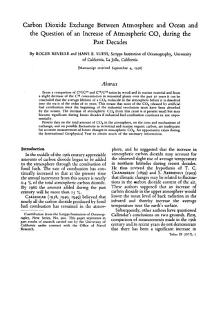
7. 24 R O G E R R E V E L L E A N D H A N S E. S U E S S
,lOyrs..
2 0 y r s
/ /’loYrs. /80
60
50 1.5% --
___) A *
UNITS of A.
Fig. I. Graphic solutions of Eq. (I a) for values ~ / k ,ranging from 10 to 80
years (straight lines), and of Eq. (5 a) for r* = 1.5 % and 1.75% (curved lines),
for average apparent C14 age of sea water ~ / k ,= 400 years (solid lines) and
300 years (broken lines). Points of intersection of straight lines and curves
are possible solutions of the two equations for effective reservoirs A* and S*.
effect from industrial fuel combustion needs
further experimental investigation.
W e conclude that the exchange time z (atm) =
=ilkl, defined as the time it takes on the average
for a CO, molecule as a member of the atmos-
pheric carbon reservoir to be absorbed by the sea,
is of the order of magnitude of 10 years. This
corresponds to a net exchange rate of the
order of IO-’ mol CO, per second and square
meter of the ocean surface, larger by a factor
of IOO than that postulated by PLASS(1956)
and smaller by a factor of IO,OOO than that
deduced by DINGLE(1954) as a lower limit
from numerical values of the various rate
controlling constants. These are, as HUTCH-
INSON (1954)has forcefully pointed out, too
uncertain to allow any definite conclusions.
On the other hand, our exchange data give a
value for the “invasion coefficient” of carbon
dioxide close to that determined experimen-
tall by BOHR (1899)for a stirred liquid
Secular variation of CO, in the atmosphere
In the preceding section of this paper, two
simplifylng assumptions were made when
surYace.
estimating the exchange rate of CO, between
the atmosphere and the oceans: (I) that the
rate constants k, and k, were not affected by a
small increase of the exchangeable carbon
reservoir such as that from industrial fuel
combustion, and (2) that, except for that
increase, no other changes in the sizes of the
oceanic and atmosphericcarbonreservoirshave
taken place. If these assumptions were rigor-
ously correct, the increase in atmosphericCO,
due to an addition of C14free CO, would be
nearly equal to r, as given by Eq. .fs) and in
table 4,and equal to the decrease in the spec&
C14 activity r*, multiplied by a factor A*/A.
Because of the peculiar buffer mechanism
of sea water, however, the increase in the
partial CO, pressure is about 10times higher
than the increase in the total CO, concentration
of sea water when CO, is added and the
alkalinity remains constant (BUCH,1933,see
also HARVEY,1955)~so that under equilibrium
conditions at a given alkalinity
y being a numerical factor of the order of 10
Tellus IX (1957), 1

8. T H E Q U E S T I O N OF I N C R E A S E OF A T M O S P H E R I C CO, 25
Fig. 2. Expected secular increase in the CO, concentration of air (7) according
to Eq. (7), for average lifetimes of COI in the atmosphere t(atm) = 10years and
3 0 years, with and without correction for the increase in the partial CO, pressure
with total CO, concentration of sea water (curves for y = 10 and y = I respec-
tively), for a constant rate of addition of industrial COPof i = 2.5 * 10-*x Ao.
for r and s small compared to A, and So
respectively.
As a reasonable ap roximation we may
write instead of Eq. (3f:
or
Figure 2 shows r as a function of time
calculated from Eq. (7) for two values of k,
corresponding to an exchange time of 10 and
30 years respectively, assuming constant addi-
tion of industrial CO, equal to 0.25 % of the
CO, in the atmosphere per year. At present
the integrated amount of industrial CO,
correspondsto about 40 to 50 years of addition
at this constant rate. The increase in CO, in
the atmosphere plus biosphere and soil due to
industrial fuel combustion should therefore at
present amount to 3 to 6 %, depending on the
assumptions made with respect to the size of
the “effective” atmos heric carbon reservoir
that exchanges with ti!e ocean.
Eq. (7) and figure 2 show that addition of
industria CO, at a constant rate should
eventually lead to a situation in which the
secular increase in CO, in the atmosphere plus. .
biosphere and soil equals __-iyk2‘k1 per year.
I -C vk,Ik.- ’ ,’-z,.-L
With So/Ao=kl/kz = 60 and i=o.zs ,an in-
crease of 3.6 % er century is obtained. We
alkalinity, which is small,comparedto the rate
have neglected tKe present rate of increase in
Tellus IX (1957). 1
of CO, production from fossil fuels. However,
over a sufficiently long period of time the
alkalinity of the ocean must be expected to rise
more rapidly as a consequence of the higher
total CO, concentrationin the atmos here and
rock weathering and to decrease the rate of
de osition of CaCO,. The secular increase in
I s1odd therefore be less than that calculated
from Eq. (7) with ~ = I Oand somewhere
between the curves shown in figure 2 for
It seems therefore quite improbable that an
increase in the atmospheric CO, concentration
of as much as 10 % could have been caused by
industrial fuel combustion during the past
century, as Calleridar’s statistical analyses
indicate. It is possible, however, that such an
increase could have taken place as the result
of a combination with various other causes.
The most obvious ones are the following:
I) Increase of the average ocean temperature
of I’ C increases Pco, by about 7 %. However,
such increase would also raise the sea level by
about 60 cm, due to thermal expansion of the
ocean water. Actually, according to MUNKand
REVELLE(1952),although the sea levelhas risen
about 10cm during the last century, this rise
can be accounted for almost quantitatively by
addition of melt water from retreating glaciers
and ice caps. The increase in the average ocean
temperatureis probably not more than 0.05’ C,
which corresponds to an increase in PCo,of
0.35 %. In the case of slow oceanic mixin ,
ocean which will tend to increase tRe rate of
y=Ioandy=I.
the increase could be somewhat larger, if oI fy

9. 26 R O G E R R E V E L L E A N D H A N S E. S U E S S
the top layers of the sea were affected by a rise
in temperature.
Z) Decrease in the carbon content of soils:
HUTCHINSON(1954) considers this the most
probable additional cause of the Callendar
effect. The increase in arable lands of about
4 x iols cm2 since the middle of the 19th
century has resulted in a corresponding
decrease of forest land of about 10%. Assuming
that 70 % of all the soil carbon is in forests
robably a considerable over-estimate), and
!Eat cultivation reduced this by so %, the
total decrease in soil carbon would correspond
to 9 x 1ol6 gms of CO, which is 4 % of that
in the atmosphere. At least four-fifths of this
amount should have been transferred to the
ocean.
3) Change in the amount of organic matter
in the oceans. About 7 % of the marine carbon
reservoir consists of organic material. The
amount of organic matter must depend on the
balance between the rates of reduction of CO,
by photosynthesis and of production of CO,
by oxidation. As pointed out previously, a
change in the CO, content of sea water by a
certain factor without a corresponding change
in alkalinity changes Pco, by about 10times
this factor. Therefore a I % change in the
concentration of organic material in the sea
will change the partial CO, pressure and hence
the atmospheric CO,,by roughly I %. During
the past 50 years, the mcrease in marine carbon
from absorption of industrial CO, of about
0.2 % might have increased the rate of photo-
synthesis without a corresponding change in
the rate of oxidation per unit mass of organic
matter, and thus decreased Pco,. An increase in
the temperature of surface water might have
increased the rate of oxidation per unit mass
of organic matter, and hence increased Pco,.
W e suspect that fluctuations in the amount of
organic marine carbon might be an important
cause for changes in the atmospheric CO,
concentration.
ERIKSONand WELANDER(1956) have dis-
cussed a mathematical model of the carbon
cycle between the atmosphere, the land bios-
phere and dead organic matter, and the ocean,
in which it is assumed that the rate of input of
carbon to the biosphere is directly proportional,
not only to the total size of the biosphere but
also to the amount of CO, in the atmosphere.
Their estimate of the land biosphere is 7 times
larger than that given in Table 3. They con-
clude that most of that part of the CO, added
by fossil fuel consumption, which has not been
absorbed by the ocean, hasybably gone into
the biosphere. Erikson an Welander’s basic
assumption that the amount of atmospheric
carbon dioxide limits the growth of the
terrestrial biosphere seems highly unlkely, in
view of the fact that the principal photo-
synthetic production on land is in forests, where
a deficiency of plant nutrients might be
expected. In any case as HUTCHINSON(1954)
has shown, the amount of carbon in the
biosphere and soil humus has probably
decreased, rather than increased, during the
past century, because of the clearing of forests.
In contemplating the probably large in-
crease in CO, production by fossil fuel
combustion in coming decades we conclude
that a total increase of 20 to 40 % in atmos-
pheric CO, can be anticipated. This should
certainly be adequate to allow a determination
of the effects, if any, of changes in atmos-
pheric carbon dioxide on weather and climate
throughout the earth.
Present data on the total amount of CO, in
the atmosphere, on the rates and mechanisms
of CO, exchange between the sea and the air
and between the air and the soils, and on
possible fluctuations in marine organic carbon,
are insufficient to give an accurate base line
for measurement of future changes in atmos-
pheric CO,. An opportunity exists during the
International Geophysical Year to obtain much
of the necessary information.
Acknowledgements
A paper on the same subject by James R.
Arnold and Ernest C. Anderson appears in this
issue of this journal; we are grateful to Drs.
Arnold and Anderson for the opportunity of
the problem before publication.
Wediscussin[are appy to note that these authors have
simultaneously and independently derived
essentially the same conclusions as presented in
this paper. W e hope that the somewhat dif-
ferent approach will make both contributions
equally valuable to the reader. We also wish to
thank Dr. Carl Eckart for valuable discussions
and Dr. Harmon Craig for much constructive
criticism. Dr. Craig’s own careful analysis of
the subject appears in a separate paper in this
issue.
Tellus IX (1957). 1

10. THE Q U E S T I O N O F I N C R E A S E O F A T M O S P H E R I C C O ,
R E F E R E N C E S
ARRHENIUS,SVANTE,1903: Lehrbuch der kosmischen Physik
2. Leipzig: Hirzel.
BOHR.C., 1899: Die Loslichkeit von Gasen in Flussig-
keiten. Ann. d. Phys. 68, p. 500.
BUCH,K., 1933: Der Borsauregehalt des Meerwassers
und seine Bedeutung bei der Berechnung des Kohlen-
sauresystems. Rapp. Cons. Explor. Mer. 85,p. 71.
CALLENDAR,G. S., 1938: The artificial production of
carbon dioxide and its influence on temperature.
Quarterly Journ. Royal Meteorol. SOL.64,p. 223.
CALLENDAR,G. S., 1940: Variations in the amount of
carbon dioxide in different air currents. Quarterly
Journ. Royal Meteorol. SOL.66,p. 395.
CALLENDAR,G. S., 1949: Can carbon dioxide influence
climate? Weather 4. p. 310.
CHAMBERLIN,T. C., 1899: An attempt to frame a working
hypothesis of the cause of glacial periods on an atmos-
pheric basis. J. oJ Geology 7, pp. 575, 667, 751.
CONWAY,E. J., 1942:Mean geochemical data in relation
to oceanic evolution. Proc. Roy. Irish Acad., B. 48,
p. 119.
CRAIG,H., 1953: The geochemistry of the stable carbon
isotopes. Geochim. et Cosmochim. Acta 3. p. 53.
CRAIG,H., 1954: Carbon 13 in plants and the relationship
between carbon 13 and carbon 14 variations in nature.
Journ. Geol. 62,p. 115.
DINGLE,H. N., 1954: The carbon dioxide exchange
between the North Atlantic Ocean and the atmos-
phere. Tellus 6, p. 342.
ERIKSON,E., and WELANDER,P., 1956: On a mathematical
model of the carbon cycle in nature. Tellus 8, p. 155.
FERGUSSON,G. J., and RAFTER,T. A.: New Zealand
C-14 Age Measurements III. In press.
FONSELIUS,S., KOROLEFF,F., and WARME,K., 1956:
Carbon dioxide variations in the atmosphere. Tellus
8, p. 176.
HARVEY,H. W., 1955: The Chemistry and Fertility of Sea
Water. Cambridge: University Press.
27
HAYES,F. N.. ANDERSON,E. C., and ARNOLD,J. R., 1955:
Liquid scintillation counting of natural radiocarbon.
Proc. of the International Conference on Peaceful Uses of
Atomic Energy, Geneva, r4. p. 188.
HUTCHINSON,G. E., 1954: In The Emth as a Planet, G.
Kuiper, ed. Chicago: University Press. Chapter 8.
MUNK,W., and REVELLE,R., 1952: Sea level and the
rotation of the earth. Am. Journ. Sci. 250, p. 829.
NIER, A. O., and GULBRANSEN,E. A., 1939: Variations in
the relative abundance of the carbon isotopes. Journ.
Am. Chem. Soc. 61,p. 697.
PLASS,G. N., 1956: Carbon dioxide theory of climatic
change. Tellus 8, p. 140.
RAFTER,T. A., 1955: C14 variations in nature and the
effect on radiocarbon dating. New ZealandJourn. Sci.
Tech. B. 37, p. 20.
RUBEY,W. W., 1951: Geologic history of sea water.
Bull. Geol. SOL.Amer. 62,p. 1111.
SLOCUM,GILES,1955: Has the amount of carbon dioxide
in the atmosphere changed significantly since the
beginning of the twentieth century?Monthly Weather
Rev. Oct., p. 22s.
SUESS,H. E., 1953: Natural Radiocarbon and the rate
of exchange of carbon ?:oxide between the atmos-
phere and the sea. Nuclear Processes in Geologic
Settings, National Academy of Sciences -National
Research Council Publication, pp. 52-56.
SIJESS,H. E., 1954: Natural radiocarbon measurements
by acetylene counting. Science 120,p. 5.
SUESS,H. E., 1955:Radiocarbon concentration in modern
wood. Science 122,p. 415.
SVERDRUP,H. U., JOHNSON,M. W., and FLEMING,R. H..
1942: The Oceans. New York: Prentice-Hall, Inc.
UNJTEDNATIONS,1955: World requirements of energy,
197j--zooo. International ConJerence on Peaceful Uses
$Atomic Energy, Geneva, I , p. 3.
UREY,H. C., 1952: The Planets. New Haven: Yale Univ.
Press.
Tellus 1X (19J7). 1