Andrew Shepherd

1. meridional transects for PCO2 measurements made
during each event are also indicated. June 1982 to
June 1983 (intense event, 1 transect); August 1986 to
July 1987 (medium, 7 transects); October 1991 to
May 1992 (marginal intensity, 2 transects); October
1992 to October 1993 (marginal, 3 transects); April
1994 to June 1995 (marginal, 8 transects); and April
1997 to April 1998 (intense, 15 transects).
12. To test biases caused by undersampling, we comput-
ed time trends of SST using the regularly spaced
monthly mean values extracted from the compilation
of Reynolds et al. (13) for the non–El Nin˜o periods
(11) in the Nin˜o 3.4 area. The SST trends thus com-
puted are compared with those computed using our
limited SST values measured concurrently with PCO2.
They are found to be in agreement within 1 SD,
indicating that the time trends computed with our
limited number and irregular spacing of measure-
ments are consistent with those obtained with the
full set of the SST data. For example, for the post-
1990 trend, the full data yield –0.14° Ϯ 0.02°C
yearϪ1
(n ϭ 87), which compares with –0.12° Ϯ
0.06°C yearϪ1
(n ϭ 32) for the most consistent case;
and for the post-1992 trend, the full data yield
–0.11° Ϯ 0.11°C yearϪ1
(n ϭ 66), which compares
with ϩ0.01° Ϯ 0.09°C yearϪ1
(n ϭ 26) for one of the
least consistent cases.
13. R. W. Reynolds, N. A. Rayner, T. M. Smith, D. C.
Stokes, W. Wang, “NOAA optimum interpolation (OI)
sea surface temperature (SST) V2” (2003) (available
at ftp://ftpprd.ncep.noaa.gov/pub/cmd/sst/papers/
oiv2pap/).
14. C. Marzban, J. T. Schaefer, Mon. Weather Rev. 129,
884 (2001).
15. W. H. Press, B. P. Flannery, S. A. Teukolsky, W. T.
Vetterling, Numerical Recipes (Cambridge Univ.
Press, Cambridge, 1986), pp. 491–494.
16. Z values greater than 2.575 indicate sufficient
evidence for claiming that the test is valid with a
greater than 99% probability.
17. T. Takahashi, J. Olafsson, J. Goddard, D. W. Chipman,
S. C. Sutherland, Global Biogeochem. Cycles 7, 843
(1993).
18. GLOBALVIEW-CO2: Cooperative Atmospheric Data In-
tegration Project—Carbon Dioxide. (CD-ROM, NOAA
Climate Monitoring and Diagnostics Laboratory,
Boulder, Colorado, 2001) (also available on Internet
via anonymous FTP to ftp.cmdl.noaa.gov. Path: ccg/
co2/GLOBALVIEW ).
19. R. L. Borgne, R. A. Feely, D. J. Mackey, Deep-Sea Res.
II 49, 2425 (2002).
20. T. P. Guilderson, D. P. Schrag, Science 281, 240
(1998).
21. D. Gu, S. G. H. Philander, Science 275, 805 (1997).
22. M. J. McPhaden, D.-X. Zhang, Nature 415, 603 (2002).
23. N. Schneider, A. J. Miller, M. A. Alexander, C. Deser, J.
Phys. Oceanogr. 29, 1056 (1999).
24. J. E. Dore, R. Lukas, D. W. Sadler, D. M. Karl, Nature
424, 764 (2003).
25. D. E. Archer et al., Deep-Sea Res. II 43, 779 (1996).
26. R. Wanninkhof, K. Thoning, Mar. Chem. 44, 189
(1993).
27. N. R. Bates, T. Takahashi, D. W. Chipman, A. H. Knapp,
J. Geophys. Res. 103, 15567 (1998).
28. D. W. Chipman, J. Marra, T. Takahashi, Deep-Sea Res.
40, 151 (1993).
29. Supported by grants from NOAA, NASA, and Ford
Motor Company (T.T.), and from NOAA (R.A.F.) for
field operations. We thank R. Wanninkhof of NOAA
and H. Y. Inoue of the Japan Meteorological Research
Institute for providing data; D. Martinson of LDEO
and C. Marzban of the Department of Statistics,
University of Washington, Seattle, for advice on sta-
tistics; and B. Linsley of the State University of New
York at Albany for critical reading of the manuscript.
This is LDEO contribution no. 6500, PMEL contribu-
tion no. 2579, and University of Washington and
Joint Institute for the Study of the Atmosphere and
Ocean contribution no. 1021.
30 June 2003; accepted 23 September 2003
Larsen Ice Shelf Has
Progressively Thinned
Andrew Shepherd,1
* Duncan Wingham,2
Tony Payne,3
Pedro Skvarca4
The retreat and collapse of Antarctic Peninsula ice shelves in tandem with
a regional atmospheric warming has fueled speculation as to how these
events may be related. Satellite radar altimeter measurements show that
between 1992 and 2001 the Larsen Ice Shelf lowered by up to 0.27 Ϯ
0.11 meters per year. The lowering is explained by increased summer melt-
water and the loss of basal ice through melting. Enhanced ocean-driven
melting may provide a simple link between regional climate warming and
the successive disintegration of sections of the Larsen Ice Shelf.
On average, Antarctic Peninsula (AP) ice
shelves have retreated by ϳ300 km2
each
year since 1980 (1). This gradual retreat has
been punctuated by two catastrophic col-
lapses, in January 1995 (2) and February
2002, when the remaining northern sections
of the Larsen Ice Shelf (LIS) (Fig. 1) frag-
mented into icebergs. In contrast to the
prolonged retreats, these 2000- and 3250-
km2
ice-shelf sections—Larsen-A and
Larsen-B—disintegrated over days or
weeks. Although the initial retreats of their
ice fronts may have resulted from iceberg
calving beyond stable geometrical posi-
tions (3), it is not clear that this explains the
wholesale disintegration of large ice-shelf
sections. Speculation as to the mechanism
that caused the final collapses has concen-
trated on the destabilizing effects of in-
creased surface melt-water (4–6), which
may have enhanced the process of crevasse
fracture (7). Although that mechanism pro-
vides a link between the regional climate
warming and the breakup of ice shelves at
the AP, direct observations are insufficient
to determine the importance of ice-shelf
stability criteria or the impact of increased
surface melt. Here, we show that the LIS
may have become susceptible to crevasse
fracture through a sustained ice thinning.
We used 9 years of European Remote
Sensing (ERS-1 and ERS-2) satellite radar
altimeter measurements to determine the
surface elevation change of the LIS since
1992. Ice-shelf surface elevation was cal-
culated relative to the WGS 84 Earth ellip-
soid at each individual crossing point of the
satellite ground track during 35-day orbit
repeat cycles (8). From these data, we
formed 45 time series of elevation change
(e.g., Fig. 2) across the LIS at the finest
resolution afforded by the ERS altimeters
(9). The ERS ground tracks provided a
mean crossing point separation of 14 km,
and the precise location of the ϳ10-km
altimeter footprint drifted by less than 1.2
km through time as a result of orbit maneu-
vers. We detected no radar penetration of
the LIS surface at any time (10), and we
removed the ocean tide from each elevation
time series using predictions of ice-shelf
tidal displacement (11). We calculated the
trend of elevation change at each crossing
point from the tide-adjusted time series and
interpolated these data using a quintic tri-
angulation scheme (Fig. 1).
Between 1992 and 2001 the mean rates
of elevation change of the Larsen-B and -C
ice shelves were –0.17 Ϯ 0.11 and –0.08 Ϯ
0.04 m yrϪ1
, respectively. In general, the
northernmost sections of the Larsen-C ex-
perienced the greatest decrease in surface
elevation, with a peak rate of lowering of
0.27 Ϯ 0.11 m yrϪ1
some 80 km west of the
Larsen meteorological station (Fig. 1). To-
ward the southern tip of Larsen-C, one time
series showed that the ice shelf thickened at
the terminus of the Lurabee Glacier
(69.25°S, 63.62°W), where ice is dis-
charged from Palmer Land. Recent radar,
seismic, and Global Positioning System el-
evation surveys (12) show that sections of
the Larsen-B lowered relative to the geoid
by 0.18 m yrϪ1
between 1991 and 1999, in
agreement with our satellite-derived rate.
The rate of elevation change of a float-
ing ice-shelf surface relative to the ellip-
soid (‫ץ‬h/‫ץ‬t) is due to fluctuations in sea-
level height (⌬s), ocean (␳w) and ice-shelf
(␳f) densities, net surface (M˙ s) and basal
(M˙ b) mass accumulation, and ice-flux di-
1
Centre for Polar Observation and Modelling, Scott
Polar Research Institute, University of Cambridge,
Cambridge CB2 1ER, UK. 2
Centre for Polar Obser-
vation and Modelling, University College London,
Gower Street, London WC1E 6BT, UK. 3
Centre for
Polar Observation and Modelling, University of
Bristol, University Road, Bristol BS8 1SS, UK. 4
In-
stituto Anta´rtico Argentino, Cerrito 1248, 1010
Buenos Aires, Argentina.
*To whom correspondence should be addressed. E-
mail: aps46@cam.ac.uk
R E P O R T S
31 OCTOBER 2003 VOL 302 SCIENCE www.sciencemag.org856
CORRECTED 12 MARCH 2004; SEE LAST PAGE

2. vergence (Mٌ.␯). For an ice column in
hydrostatic equilibrium with no vertical ice
shear, ‫ץ‬h/‫ץ‬t can be written as
‫ץ‬h
‫ץ‬t
ϭ
‫⌬ץ‬s
‫ץ‬t
– M
‫ץ‬
‫ץ‬tͩ1
␳w
ͪϩ ͵0
M
dm
‫ץ‬
‫ץ‬tͩ 1
␳f (m)ͪϩ
ͩ 1
␳ice – ␳w
ͪ(M˙ s ϩ M˙ b ϩ Mٌ.␯) (1)
where ␳ice is the density of ice (917 kg mϪ3
)
and M is the ice-shelf mass per unit area. We
investigated trends and variability in each
component of Eq. 1 to determine the origin of
the LIS surface lowering.
External contributions to ‫ץ‬h/‫ץ‬t include
sea level and density. Although eustatic sea
level has risen by only 2 mm yrϪ1
in the
20th century (13), atmospheric pressure
fluctuations occur (14) that could lead to a
9-year uncertainty in ⌬s of up to 11 mm
yrϪ1
. Tide model inaccuracies introduce a
further 26 mm yrϪ1
uncertainty. Oceano-
graphic records show that seasonal and in-
terannual variations in salinity (15) modify
␳w, resulting in up to 10 mm yrϪ1
uncer-
tainty in elevation change. In addition,
nearby deep and surface layers of the Wed-
dell Sea have warmed by 0.01°C yrϪ1
for
several decades (16, 17), and a similar
warming (or cooling) of the water beneath
the LIS could raise (or lower) the ice shelf
at a rate of 15 mm yrϪ1
. We estimate the
combined uncertainty resulting from these
contributions to be 34 mm yrϪ1
, a value
that is small when compared with the ob-
served trend. The LIS lowering must reflect
a change in the ice shelf itself.
We investigated the possibility that the
LIS ‫ץ‬h/‫ץ‬t may have resulted from a mass-
conservative densification of the ice shelf
(the third term in Eq. 1). The gradually warm-
ing (18) and lengthening (19) summer cli-
mate may have accelerated firn densification
during the interval of the measurement. To
bound this acceleration, we estimated an ini-
tial LIS firn density (20) and supposed that
the entire upper 8 m of firn layer (beneath
which interannual temperature changes do
not penetrate) (12) were densified to ice. This
calculation leads to rates of elevation change
of –0.12 and –0.28 m yrϪ1
at the Larsen-B
and -C, respectively, the difference reflecting
the lower initial density of the colder Larsen-
C. These changes are comparable to the ob-
served lowering (Fig. 1), and densification
cannot be excluded as the sole explanation of
the lowering. However, the energy available
for thermally driven firn densification is lim-
ited by air temperature (1) and melt-season
duration (19), which decrease southward. We
used observed ablation measurements and a
positive degree-day model (21) to estimate
the change in summer melt-water production
(22). Assuming the increased melt-water is
entirely retained at the density of ice, the
estimated contribution to ‫ץ‬h/‫ץ‬t was –0.07 and
–0.05 m yrϪ1
at the Larsen-B and -C, respec-
tively. To assign all of the observed lowering
of the Larsen-C to densification makes a
heavy demand on melt-water production
(Fig. 3) at the northern Larsen-C.
To investigate further, we examined in
detail airborne measurements of Larsen-C ice
thickness that have been ongoing for several
decades (23). These data show that the
Larsen-C has thinned at an average rate of
0.29 Ϯ 0.68 m yrϪ1
since 1966 (24). Al-
though the aircraft data are sparse and uncer-
tain, this rate shows that the thinning predates
for several decades that observed more pre-
cisely by the satellite. Allocating this rate to
densification, for which the thinning rate
equals the elevation rate relative to sea level,
appears incompatible with the trend in melt-
water production (22). Our conclusion is that,
for Larsen-C at least, some other cause of
thinning is present as well.
The remaining terms in Eq. 1 are mass
losses. A 10% centuryϪ1
increase in snow ac-
cumulation (M˙ s) similar to that recorded nearby
at the ϳ2000-m altitude Dyer Plateau (25)
would increase surface elevation by some 2 mm
yrϪ1
. Fluctuations occur at shorter time scales
(8), but snow-pit measurements at Larsen-B
show that accumulation has remained close to
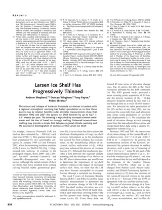
Fig. 1. Rate of surface elevation
change of the Larsen Ice Shelf
determined from ERS radar al-
timeter measurements recorded
between 1992 and 2001 (color
scale and 0.1 m yrϪ1
white con-
tours). The elevation data are
superimposed on a mosaic of
Advanced Very-High-Resolution
radiometer (AVHRR) satellite
imagery (gray scale) (38), and
data points used in the interpo-
lation are shown as black dots.
Also shown are the locations of
meterological stations (blue
dots) and stakes used to mea-
sure changes in snow height (red
dots) and surface mass balance
(5-km grid, centered at green
dot). The 1990 boundaries of the
Larsen-A, -B, and -C ice-shelf
sections are highlighted with
blue, green, and red borders, re-
spectively. Larsen-A collapsed
before the ERS measurements;
Larsen-B has since disintegrated;
Larsen-C remains intact.
Fig. 2. Change in surface elevation between 1992 and 2001 recorded by the ERS radar altimeters
ϳ80 km west of the Larsen meteorological station (see Fig. 1) at the Larsen-C ice shelf before (A)
and after (B) removal of the periodic signal of ocean tide (11). On average, the tide correction
reduced the variability in the trends from 0.4 to 0.2 m yrϪ1
. The location of this time series is
highlighted with a white border in Fig. 1.
R E P O R T S
www.sciencemag.org SCIENCE VOL 302 31 OCTOBER 2003 857

3. the long-term average (26), with a 9-year vari-
ability of 31 mm yrϪ1
. Turning to the mass
supply (M), reduced glacier influx must have
occurred for the advection time scale of 102
to
103
years to affect the entire LIS. However,
ice-core records show no accumulation deficit
within the catchment basins of tributary glaciers
(25), and there is no reason to suppose that
these glaciers have thinned. It is possible that a
warming of the shelf interior, or a reduction
in stress at pinning points, may have dis-
turbed the LIS force balance (3) and thus ٌ.␯.
We constructed a two-dimensional model of
the LIS based on the standard rheology equa-
tions and momentum and mass-continuity
equations (27, 28), to determine, as an exam-
ple, the effect of a decrease in ice-shelf
viscosity. We determined the thinning asso-
ciated with a 2°C warming penetrating to
different depths, and the maximum lowering
rate that could be attained was 8 mm yrϪ1
,
because of the slow response to changes in
the force balance. The combined uncertainty
of all of these estimates is 32 mm yrϪ1
. Any
LIS mass imbalance must have arisen
through basal melting (M˙ b).
Although basal melting rates under the
LIS are uncertain and their fluctuation even
more so, the conclusion that basal melting
has been and is thinning the LIS, at an aver-
age rate our measurement and estimate of the
effect of densification (Fig. 3) put at 0.78 m
yrϪ1
, is not unreasonable given the oceano-
graphic data. Beneath the nearby Filchner-
Ronne Ice Shelf (FRIS), melt rates are typi-
cally 0.19 m yrϪ1
(29), but substantially
greater melt occurs in regions where warm
waters are transported beneath floating ice
(30). Basal melt rates of 2 to 3 m yrϪ1
are
observed up to 200 km inshore of the FRIS
ice front, where tidal mixing occurs (29). On
average, nearby Weddell Sea Deep Waters
(WDW) have warmed by 0.32°C since 1972
(16). In 2002, oceanographic measurements
showed large quantities of modified WDW
present in front of the northern Larsen-C
(66.5°S) at depths well below the ice-shelf
draft (300 m), with a potential temperature of
–1.45 °C, that is, 0.65°C higher than the
pressure melting point of ice (31). Elsewhere
such differences generate up to 6.5 m yrϪ1
of
basal ice melt (30) when water is delivered to
the ice-shelf base.
The calving front of the Larsen-C has
changed little in decades, and its flow ge-
ometry is considered to be stable (3). How-
ever, at the same time enhanced ocean
melting has progressively thinned the shelf
at its base. Thinning inevitably increases
the ice-shelf exposure to crevasse fracture
(7), and it is difficult to conclude that the
thinning did not contribute toward either
the creation of unstable conditions or the
final disintegrations of the Larsen-A and -B
sections. If our estimate of the basal ero-
sion rate is correct, the Larsen-C will ap-
proach the thickness of the Larsen-B at the
time of its collapse in some 100 years, more
rapidly if the rate is increased by a warming
ocean. It is possible that the LIS thinning
provides a link between the regional cli-
mate warming and the disintegration of ice
shelves at the Antarctic Peninsula.
References and Notes
1. D. G. Vaughan, C. S. M. Doake, Nature 379, 328
(1996).
2. H. Rott, P. Skvarca, T. Nagler, Science 271, 788 (1996).
3. C. S. M. Doake, H. F. J. Corr, H. Rott, P. Skvarca, N. W.
Young, Nature 391, 778 (1998).
4. J. H. Mercer, Nature 271, 321 (1978).
5. H. Rott, W. Rack, T. Nagler, P. Skvarca, Ann. Glaciol.
27, 86 (1998).
6. T. A. Scambos, C. Hulbe, M. Fahnestock, J. Bohlander,
J. Glaciol. 46, 516 (2000).
7. J. Weertman, International Association of Scientific
Hydrology Publication 95, 139 (1973).
8. D. J. Wingham, A. Ridout, R. Scharroo, R. Arthern, C. K.
Shum, Science 282, 456 (1998).
9. A. Shepherd, D. J. Wingham, J. A. D. Mansley, H. F. J.
Corr, Science 291, 862 (2001).
10. Changes in the electromagnetic properties of ice
surfaces can affect the elevation recorded by a
radar altimeter, and the shape of radar echoes
reflects the degree of wave penetration (32). We
examined radar echoes from the LIS in detail, and
they were almost identical to those reflected from
an ocean surface. Analytical fits of a surface scat-
tering model (33) to each time series of radar
echoes yielded high correlation coefficients (r 2
Ͼ
0.96) in all instances. We detected no temporal
change in the echoes and no penetration of the
surface layer at any time.
11. Ocean tides generate up to 2.5 m of vertical
motion at the LIS (34). Station data are too remote
to produce tidal predictions for the entire LIS, and
ocean tide solutions can prove inaccurate for ice
shelves that do not respond freely to tidal forcing
(35). We derived a model of the LIS tidal motion
from the ERS altimeter data set itself (36) to
estimate the displacement at the time and location
of each elevation measurement. The same model
resolved the four principal tidal constituents to
within 10.9 cm of station records at the George VI
Ice Shelf, ϳ500 km southeast.
12. W. Rack, thesis, Leopold-Franzens-Universitat
(2000).
13. R. Warwick, C. Le Provost, M. Meier, J. Oerlemans, P.
Woodworth, in Climate Change 1995: The Science of
Climate Change (Cambridge Univ. Press, Cambridge,
1996), pp. 359–405.
14. J. R. Potter, J. G. Paren, M. Pedley, British Antarctic
Survey Bulletin 68, 1 (1985).
15. M. J. Whitehouse, J. Priddle, C. Symon, Deep-Sea
Research Part I–Oceanographic Research Papers 43,
425 (1996).
16. R. Robertson, M. Visbeck, A. L. Gordon, E. Fahrback,
Deep Sea Research 49, 4791 (2002).
17. J. C. Comiso, Journal of Climate 13, 1674 (2000).
18. D. G. Vaughan, G. J. Marshall, W. M. Connolley, J. C.
King, R. Mulvaney, Science 293, 1777 (2001).
19. M. A. Fahnestock, W. Abdalati, C. A. Shuman, Ann.
Glaciol. 34, 127 (2002).
20. Firn density at the northern margin of the Larsen-B
exceeds 838 kg mϪ3
at ϳ0.5 m depths (12). De-
tailed measurements on the George VI ice shelf, on
the western coast of the AP, which has a melt
season and temperature similar to those of the LIS,
show values of ϳ900 kg mϪ3
in regions of melt
ponding (similar to the northern LIS) and ϳ600 kg
mϪ3
elsewhere (37). We use this latter value as a
lower bound for the LIS surface density, the values
measured in situ at the northern Larsen-B, and the
latitudinal variation in annual melt-water produc-
tion (22) to model the spatial variation in LIS
surface firn density. This calculation gives surface
density values of 893, 793, and 630 kg mϪ3
for the
Larsen-A, -B and -C ice shelves, respectively.
21. N. Reeh, Polarforschung 59, 113 (1991).
22. A comparison of surface ablation measurements re-
corded at five stakes (see Fig. 1) between 1996 and
2002 and positive degree-days recorded at meteoro-
logical stations to the north (Marambio) and south
(Larsen) shows that average ablation equaled 2.8 Ϯ
1.0 mm water-equivalent degree-dayϪ1
. We used
this factor and a positive degree-day model (21) to
estimate changes in the mass of melted firn (table
S1). Melt-water production was much larger at
northerly latitudes.
23. M. B. Lythe, D. G. Vaughan, J. Geophys. Res. 106,
11335 (2001).
24. More than 115,000 direct measurements of ice
thickness have been recorded at the LIS on 11
separate occasions since 1966 (23). Absolute loca-
tion and ice-thickness precision varied from 0.5 to
5000 m and 3 to 30 m, respectively, with older
data showing the greatest uncertainty. We inter-
polated the entire 32-year, irregularly oriented
ice-thickness data set onto a 500-m grid to facil-
itate coregistration and isolated more than 1000
separate locations where repeat measurements co-
incided. Some data were discarded in regions of
high surface roughness. The 1966 to 1998 mean
rate of thickness change of the Larsen-C ice-shelf
was –0.29 Ϯ 0.68 m yrϪ1
.
25. C. Raymond et al., J. Glaciol. 42, 510 (1996).
26. J. Turner, S. Leonard, T. Lachlan-Cope, G. J. Marshall,
J. Glaciol. 27, 591 (1998).
27. W. S. B. Paterson, The Physics of Glaciers (Butter-
worth-Heinemann, Oxford, ed. 3, 1994).
28. K. Herterich, in Dynamics of the West Antarctic Ice
Fig. 3. Larsen Ice Shelf (LIS) surface elevation
change (diamonds) along transect A-B (Fig. 1),
compared with the estimated change due to in-
creased melt-water production (22). The model
assumes that melt-water mass is conserved by
the shelf (solid line) until an initial 8-m layer
densifies to ice, in which case the excess is sup-
posed to run off (dashed line). No runoff occurs
from the LIS section included in our satellite data
set. Although stake measurements at Larsen-B
(see Fig. 1) show large increases in surface melt-
ing—in line with the model prediction—they say
nothing about conditions farther south. Our data
show that a 31,000-km2
region of the LIS be-
tween 65.5°S and 67.5°S lowered by 0.08 Ϯ
0.03 m yrϪ1
more than the rate expected from
densification, equivalent to the freeboard expres-
sion of a 21 Ϯ 8 gigaton yrϪ1
loss of ice mass.
R E P O R T S
31 OCTOBER 2003 VOL 302 SCIENCE www.sciencemag.org858

4. Sheet, C. J. Van der Veen, J. Oerlemans, Eds. (Reidel,
Dordrecht, 1987).
29. I. Joughin, L. Padman, Geophys. Res. Lett. 30, 1477
(2003).
30. E. Rignot, S. S. Jacobs, Science 296, 2020 (2002).
31. K. Nicholls, personal communication.
32. J. K. Ridley, K. C. Partington, International Journal of
Remote Sensing 9, 601 (1988).
33. G. S. Brown, IEEE Transactions of Antennas and Prop-
agation 25, 67 (1977).
34. J. O. Speroni, W. C. Dragani, E. E. D’Onofrio, M. R.
Drabble, C. A. Mazio, Geoactas 25, 1 (2001).
35. N. Reeh, C. Mayer, O. B. Olesen, E. L. Christensen,
H. H. Thomsen, Ann. Glaciol. 31, 111 (2000).
36. A. Shepherd, N. R. Peacock, J. Geophs. Res. 108, 3198
(2003).
37. C. S. M. Doake, Ann. Glaciol. 5, 47 (1984).
38. J. G. Ferrigno et al., AVHRR Antarctic Mosaic (USGS
I-2560, 2001).
39. Supported by the United Kingdom Natural Environment
Research Council Centre for Polar Observation and
Modelling and Instituto Anta´rtico Argentino. We thank
the European Space Agency for ERS data and the British
Antarctic Survey for access to the BEDMAP database.
We also thank J. Mansley, H. De Angelis, and G. Marshall
for assistance with data collection and processing, and
D. Vaughan and E. Morris for their valuable comments.
Supporting Online Material
www.sciencemag.org/cgi/content/full/302/5646/856/
DC1
Table S1
29 July 2003; accepted 23 September 2003
Carbonate Deposition, Climate
Stability, and Neoproterozoic
Ice Ages
Andy J. Ridgwell,1
* Martin J. Kennedy,1
Ken Caldeira2
The evolutionary success of planktic calcifiers during the Phanerozoic stabilized
the climate system by introducing a new mechanism that acts to buffer ocean
carbonate-ion concentration: the saturation-dependent preservation of car-
bonate in sea-floor sediments. Before this, buffering was primarily accom-
plished by adjustment of shallow-water carbonate deposition to balance oce-
anic inputs from weathering on land. Neoproterozoic ice ages of near-global
extent and multimillion-year duration and the formation of distinctive sedi-
mentary (cap) carbonates can thus be understood in terms of the greater
sensitivity of the Precambrian carbon cycle to the loss of shallow-water en-
vironments and CO2-climate feedback on ice-sheet growth.
The growth of continental-scale ice sheets ex-
tending to the tropics during the second half of
the Neoproterozoic (1000 to 540 million years
ago) (1) is now widely accepted in the geolog-
ical community and has been of particular in-
terest because of its close stratigraphic associa-
tion with the first appearance of metazoans and
the possibility that ice ages served as an envi-
ronmental filter for animal evolution (2). The
severity of these ice ages, which may record the
coldest times in Earth history (3), implies that
the Precambrian climate system must have op-
erated very differently from today. This is sup-
ported by the ubiquitous occurrence of thin
post-glacial “cap” carbonate units (4–7), appar-
ent perturbations of the carbon cycle that did
not recur in the Phanerozoic. To account for
these observations, we focus on a first-order
difference between the Precambrian and mod-
ern Earth systems and its implications for
atmospheric CO2: the absence of a well-
developed deep-sea carbonate sink before the
proliferation of calcareous plankton.
On the time scale of glaciations (ϳ104
to
106
years), the balance between weathering of
terrigenous rocks and the burial flux of calcium
carbonate (CaCO3) in marine sediments exerts
a key control on ocean carbonate chemistry (8),
with this burial today divided roughly equally
between deep-water (pelagic) and shallow-
water (neritic) zones (9). The latter sink is of
particular relevance in the context of ice ages,
because the total neritic area available for
CaCO3 burial is highly sensitive to sea level, a
consequence of the nonuniform distribution of
the Earth’s surface area with elevation (Fig. 1).
The climatic relevance arises because any in-
crease in the carbonate ion concentration
([CO3
2–
]) at the ocean surface will induce lower
atmospheric CO2 (because the aqueous carbon-
ate equilibrium, CO2 ϩ CO3
2–
ϩ H2O 7
2HCO3
–
, is shifted to the right). This is the
basis for the coral reef hypothesis for Quater-
nary glacial-interglacial CO2 control (10–13),
in which lowered sea level reduces available
neritic area and CaCO3 accumulation rates,
driving higher [CO3
2–
] and lower CO2.
We have identified a fundamental differ-
ence between ancient and modern carbon cy-
cles in the relative importance of the neritic
carbonate sink that would make the impact of a
coral reef–like effect much greater in the Pre-
cambrian. In the modern system, higher
[CO3
2–
] enhances the preservation of carbonate
in deep-sea sediments; hence, a reduction in
neritic carbonate deposition due to a fall in sea
level can be compensated for by a greater burial
flux in deep-sea sediments of CaCO3 that orig-
inates from planktic calcifiers (9) (Fig. 1). This
provides a strong negative (stabilizing) feed-
back on the modern carbon cycle, restricting
oceanic [CO3
2–
] variation and thus limiting the
atmospheric response to sea level change.
The Neoproterozoic carbon cycle, by con-
trast, did not possess this stabilizing feedback,
because before the advent of pelagic calcifiers in
the Cambrian and the subsequent proliferation
of coccolithophores and foraminifera during the
Mesozoic (14), carbonate deposition would
have been largely limited to neritic zones. The
importance of the calcareous plankton that dom-
inate carbonate deposition in the modern open
ocean (9) is illustrated by the comparative rarity
of deep-sea pelagic carbonate material in ophio-
lite suites older than ϳ300 million years (14).
As neritic carbonate deposition was the domi-
nant mechanism of CO3
2–
removal in the Pre-
cambrian ocean, it follows that atmospheric
CO2 would have been much more sensitive to
sea level change. We explore the implications
for the Neoproterozoic carbon cycle of sea level
variation with the aid of a numerical model (15).
This model calculates the evolution in atmo-
spheric CO2 that arises from a reduction in the
area available for neritic carbonate deposition.
Although these observational and evolution-
ary arguments suggest a highly limited role for
the deep-sea carbonate buffer in the Precam-
brian carbon cycle, Precambrian ocean chemis-
try would instead have been stabilized by the
dependence of shallow-water carbonate deposi-
tion rates on [CO3
2–
] (8). As oceanic [CO3
2–
]
(and saturation state, ⍀) rises after a fall in sea
level, the smaller area available for carbonate
deposition is eventually compensated for by a
higher precipitation rate per unit area. An anal-
ogous compensating increase in the neritic
CaCO3 precipitation rate may have occurred at
the Cretaceous/Tertiary boundary after the ex-
tinction-driven reduction of pelagic carbonate
productivity (8). The precipitation rate of car-
bonate minerals is expressed in the model as a
proportionality with (⍀ – 1)n
(16), where ⍀ is
defined as ([Ca2ϩ
] ϫ [CO3
2–
])/Ksp (where Ksp
is a solubility constant). The parameter n is a
measure of how strongly CaCO3 precipitation
rate responds to a change in ambient [CO3
2–
]
and thus of how effectively ocean chemistry
and atmospheric CO2 are buffered. Possible
values range from ϳ1.0 for modern biological
systems such as corals (17) to 1.9 Յ n Յ 2.8 for
precipitation that occurs under entirely abiotic
conditions (16). We therefore initially set n ϭ
1.7 (8, 11). Because CaCO3 precipitation dur-
1
Department of Earth Sciences, University of
California–Riverside, Riverside, CA 92521, USA.
2
Climate and Carbon Cycle Modeling Group, Lawrence
Livermore National Laboratory, 7000 East Avenue,
L-103, Livermore, CA 94550, USA.
*To whom correspondence should be addressed. E-
mail: andyr@citrus.ucr.edu
R E P O R T S
www.sciencemag.org SCIENCE VOL 302 31 OCTOBER 2003 859

5. 1www.sciencemag.org SCIENCE Erratum post date 12 MARCH 2004
post date 12 March 2004
ERRATUM
C O R R E C T I O N S A N D C L A R I F I C A T I O N S
RREEPPOORRTTSS:: “Larsen Ice Shelf has progressively thinned” by A. Shepherd
et al. (31 Oct. 2003, p. 856). There were two errors in the printed
form of equation (1): an incorrect expression of the density-related
factor of the mass fluctuation terms and an incorrect expression of
the mass flux divergence. The correct equation, which the authors
used in their analysis, appears below.
The authors thank David Holland for bringing these errors to their at-
tention.
∂
∂
=
∂
∂
−
∂
∂





 +
∂
∂ ( )






+ −





 + + ∇( )∫
h
t t
M
t
dm
t m
M M Mvs
w f
M
ice w
s b
∆ 1 1 1 1
0
ρ ρ ρ ρ
˙ ˙ .( )