process control

1. Chapter
14
1
Closed-Loop Frequency Response and
Sensitivity Functions
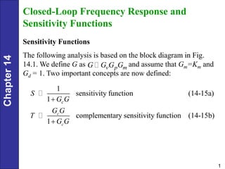
Sensitivity Functions
The following analysis is based on the block diagram in Fig.
14.1. We define G as and assume that Gm=Km and
Gd = 1. Two important concepts are now defined:
v p m
G G G G
1
sensitivity function (14-15a)
1
complementary sensitivity function (14-15b)
1
c
c
c
S
G G
G G
T
G G



2. Chapter
14
2
Comparing Fig. 14.1 and Eq. 14-15 indicates that S is the
closed-loop transfer function for disturbances (Y/D), while T is
the closed-loop transfer function for set-point changes (Y/Ysp). It
is easy to show that:
1 (14-16)
S T
 
As will be shown in Section 14.6, S and T provide measures of
how sensitive the closed-loop system is to changes in the
process.
• Let |S(j )| and |T(j )| denote the amplitude ratios of S and T,
respectively.
• The maximum values of the amplitude ratios provide useful
measures of robustness.
• They also serve as control system design criteria, as discussed
below.
ω ω

3. Chapter
14
3
• Define MS to be the maximum value of |S(j )| for all
frequencies:
ω
ω
max | ( ω) | (14-17)
S
M S j
The second robustness measure is MT, the maximum value of
|T(j )|:
ω
ω
max | ( ω) | (14-18)
T
M T j
MT is also referred to as the resonant peak. Typical amplitude
ratio plots for S and T are shown in Fig. 14.13.
It is easy to prove that MS and MT are related to the gain and
phase margins of Section 14.4 (Morari and Zafiriou, 1989):
1 1
GM , PM 2sin (14-19)
1 2
S
S S
M
M M
  
   
  

4. Chapter
14
4
Figure 14.13 Typical S and T magnitude plots. (Modified from
Maciejowski (1998)).
Guideline. For a satisfactory control system, MT should be in the
range 1.0 – 1.5 and MS should be in the range of 1.2 – 2.0.

5. Chapter
14
5
It is easy to prove that MS and MT are related to the gain and
phase margins of Section 14.4 (Morari and Zafiriou, 1989):
1 1
GM , PM 2sin (14-19)
1 2
S
S S
M
M M
  
   
  
1
1 1
GM 1 , PM 2sin (14-20)
2
T T
M M
  
    
 

6. Chapter
14
6
Bandwidth
• In this section we introduce an important concept, the
bandwidth. A typical amplitude ratio plot for T and the
corresponding set-point response are shown in Fig. 14.14.
• The definition, the bandwidth ωBW is defined as the frequency at
which |T(jω)| = 0.707.
• The bandwidth indicates the frequency range for which
satisfactory set-point tracking occurs. In particular, ωBW is the
maximum frequency for a sinusoidal set point to be attenuated
by no more than a factor of 0.707.
• The bandwidth is also related to speed of response.
• In general, the bandwidth is (approximately) inversely
proportional to the closed-loop settling time.

7. Chapter
14
7
Figure 14.14 Typical closed-loop amplitude ratio |T(jω)| and
set-point response.

8. Chapter
14
8
Closed-loop Performance Criteria
Ideally, a feedback controller should satisfy the following
criteria.
1. In order to eliminate offset, |T(jω)| 1 as ω  0.
2. |T(jω)| should be maintained at unity up to as high as
frequency as possible. This condition ensures a rapid
approach to the new steady state during a set-point change.
3. As indicated in the Guideline, MT should be selected so that
1.0 < MT < 1.5.
4. The bandwidth ωBW and the frequency ωT at which MT
occurs, should be as large as possible. Large values result in
the fast closed-loop responses.
Nichols Chart
The closed-loop frequency response can be calculated analytically
from the open-loop frequency response.

9. Chapter
14
9
Figure 14.15 A Nichols chart. [The closed-loop amplitude ratio
ARCL ( ) and phase angle are shown in families
of curves.]
 
φCL   

10. Chapter
14
10
Example 14.8
Consider a fourth-order process with a wide range of time
constants that have units of minutes (Åström et al., 1998):
1
(14-22)
( 1)(0.2 1)(0.04 1)(0.008 1)
v p m
G G G G
s s s s
 
   
Calculate PID controller settings based on following tuning
relations in Chapter 12
a. Ziegler-Nichols tuning (Table 12.6)
b. Tyreus-Luyben tuning (Table 12.6)
c. IMC Tuning with (Table 12.1)
d. Simplified IMC (SIMC) tuning (Table 12.5) and a second-
order plus time-delay model derived using Skogestad’s model
approximation method (Section 6.3).
τ 0.25 min
c 

11. Chapter
14
11
Determine sensitivity peaks MS and MT for each controller.
Compare the closed-loop responses to step changes in the set-
point and the disturbance using the parallel form of the PID
controller without a derivative filter:
( ) 1
1 τ (14-23)
( ) τ
c D
I
P s
K s
E s s
 

  
 
 
Assume that Gd(s) = G(s).

12. Chapter
14
12
Controller Kc MS MT
Ziegler-
Nichols
18.1 0.28 0.070 2.38 2.41
Tyreus-
Luyben
13.6 1.25 0.089 1.45 1.23
IMC 4.3 1.20 0.167 1.12 1.00
Simplified
IMC
21.8 1.22 0.180 1.58 1.16
τ (min)
I τ (min)
D
Controller Settings for Example 14.8

13. Chapter
14
13
Figure 14.16 Closed-loop responses for Example 14.8. (A set-
point change occurs at t = 0 and a step disturbance at t = 4 min.)