![A 1-D Growth Model for Low Speed Jets PRESENTED TO Dr. A. BENARD BY ANUPAM DHYANI As a requirement for the partial completion of ME 872 [ F E M]](https://image.slidesharecdn.com/a1dbreakupmodelfor-124355935197-phpapp02/85/A-1-D-Breakup-Model-For-1-320.jpg)
![A 1-D Growth Model for Low Speed Jets PRESENTED TO Dr. A. BENARD BY ANUPAM DHYANI As a requirement for the partial completion of ME 872 [ F E M]](https://image.slidesharecdn.com/a1dbreakupmodelfor-124355935197-phpapp02/75/A-1-D-Breakup-Model-For-1-2048.jpg)
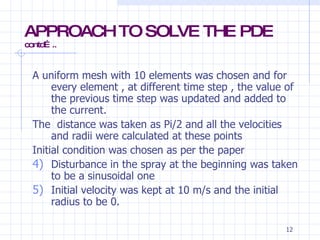
![APPROACH TO SOLVE THE PDE A Semi-explicit time marching approach is used to solve the governing equations numerically. The Equations (3) & (4) were solved for each time step using the algorithm: u(x,t n+1 ) = u(x,t n ) + ½[ ( u/ t) x,tn + ( u/ t) x,t n+1 ] t ……..(5) R(x,t n+1 ) = R(x,t n ) + ½[ ( R/ t) x,tn + ( R/ t) x,t n+1 ] t …….(6) At each time step, all variables and their derivatives at time n +1 were set to be the values at time step n before iteration. The values at time n +1 were updated during the iteration.](https://image.slidesharecdn.com/a1dbreakupmodelfor-124355935197-phpapp02/85/A-1-D-Breakup-Model-For-8-320.jpg)
![APPROACH TO SOLVE THE PDE contd….. The equations are already discretized and can be solved by using the Euler First Order Unwinding [U j n+1 – U j n ]/ t + c [U j n – U j-1 n ]/ x =0 if c>0 It is a simple one step method. This scheme is explicit as only one unknown is present in each equation.](https://image.slidesharecdn.com/a1dbreakupmodelfor-124355935197-phpapp02/85/A-1-D-Breakup-Model-For-9-320.jpg)
![APPROACH TO SOLVE THE PDE contd….. since in the equations (5) & (6) the U and R do not change in space only at different time steps this technique was implemented U(x,t n+1 ) = u(x,t n ) + ½ [(u j n -u j n-1 )/ t + (u j n+1 - u j n )/ t] t U(x,t n+1 ) = u(x,t n ) + ½ [(u j n+1 -u j n-1 )/ t] t u j n+1 = u j n + ½[(u j n+1 - u j n-1 )] u j n+1 = 2*[u j n - ½ u j n-1 )]](https://image.slidesharecdn.com/a1dbreakupmodelfor-124355935197-phpapp02/85/A-1-D-Breakup-Model-For-10-320.jpg)
![APPROACH TO SOLVE THE PDE contd….. And similarly for Radius R R(x,t n+1 ) = R(x,t n ) + ½ [(R j n -R j n-1 )/ t + (R j n+1 - R j n )/ t] t R(x,t n+1 ) = R(x,t n ) + ½ [( R j n+1 -R j n-1 )/ t] t R j n+1 = R j n + ½[(R j n+1 - R j n-1 )] R j n+1 = 2*[R j n - ½ R j n-1 )]](https://image.slidesharecdn.com/a1dbreakupmodelfor-124355935197-phpapp02/85/A-1-D-Breakup-Model-For-11-320.jpg)
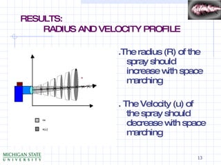
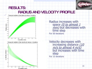


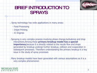
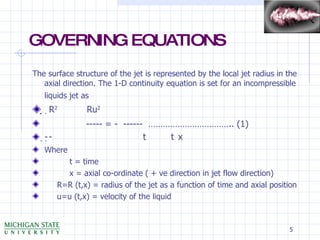
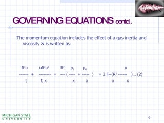
This document presents a 1-D growth model for low-speed jets in the context of spray technology, highlighting its applications in food processing, inkjet printing, and IC engines. It discusses various breakup models critical to understanding the primary breakup of sprays and outlines the governing equations used to analyze jet behavior. Numerical methods, including a semi-explicit time marching approach, are detailed for solving the governing equations, with results showing how radius and velocity profile change over space and time.