Machine design fatigue load

1. Fatigue Loading

2. Nature of fatigue failure
 Starts with a crack
 Usually at a stress concentration
 Crack propagates until the material fractures
suddenly
 Fatigue failure is typically sudden and
complete, and doesn’t give warning

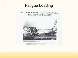
3. Fatigue Failure Examples
 Various Fatigue Crack Surfaces
 Bolt Fatigue Failure
 Drive AISI 8640 Pin
 Steam Hammer Piston Rod

4. Fatigue Example 1

5. Fatigue Failure Example

6. Fatigue Failure Example

7. Fatigue Failure Example

8. Stamping Fatigue Failure Example

9. 

10. Seat Fatigue Failure

11. Fatigue
 Fatigue strength and endurance limit
 Estimating FS and EL
 Modifying factors
 Thus far we’ve studied static failure of machine elements
 The second major class of component failure is due to dynamic loading
 Variable stresses
 Repeated stresses
 Alternating stresses
 Fluctuating stresses
 The ultimate strength of a material (Su) is the maximum stress a
material can sustain before failure assuming the load is applied only
once and held
 A material can also fail by being loaded repeatedly to a stress level that
is LESS than Su
 Fatigue failure

12. Approach to fatigue failure in analysis and design
 Fatigue-life methods (6-3 to 6-6)
 Stress Life Method (Used in this course)
 Strain Life Method
 Linear Elastic Fracture Mechanics Method
 Stress-life method (rest of chapter 6)
 Addresses high cycle Fatigue (>103 ) Well
 Not Accurate for Low Cycle Fatigue (<103)

13. The 3 major methods
 Stress-life
 Based on stress levels only
 Least accurate for low-cycle fatigue
 Most traditional
 Easiest to implement
 Ample supporting data
 Represents high-cycle applications adequately
 Strain-life
 More detailed analysis of plastic deformation at localized regions
 Good for low-cycle fatigue applications
 Some uncertainties exist in the results
 Linear-elastic fracture mechanics
 Assumes crack is already present and detected
 Predicts crack growth with respect to stress intensity
 Practical when applied to large structures in conjunction with computer
codes and periodic inspection

14. Fatigue analysis
 2 primary classifications of
fatigue
 Alternating – no DC component
 Fluctuating – non-zero DC
component

15. Analysis of alternating stresses
 As the number of cycles
increases, the fatigue strength
Sf (the point of failure due to
fatigue loading) decreases
 For steel and titanium, this
fatigue strength is never less
than the endurance limit, Se
 Our design criteria is:
 As the number of cycles
approaches infinity (N  ∞),
Sf(N) = Se (for iron or Steel)
a
f N
S




)
(

16. Method of calculating fatigue strength
 Seems like we should be able to use graphs
like this to calculate our fatigue strength if
we know the material and the number of
cycles
 We could use our factor of safety equation
as our design equation
 But there are a couple of problems with this
approach
 S-N information is difficult to obtain and thus is
much more scarce than -e information
 S-N diagram is created for a lab specimen
 Smooth
 Circular
 Ideal conditions
 Therefore, we need analytical methods for
estimating Sf(N) and Se
a
f N
S




)
(

17. Terminology and notation
 Infinite life versus finite life
 Infinite life
 Implies N ∞
 Use endurance limit (Se) of material
 Lowest value for strength
 Finite life
 Implies we know a value of N (number of cycles)
 Use fatigue strength (Sf) of the material (higher than Se)
 Prime (‘) versus no prime
 Strength variable with a ‘ (Se’)
 Implies that the value of that strength (endurance limit) applies to a LAB SPECIMEN in
controlled conditions
 Variables without a ‘ (Se, Sf)
 Implies that the value of that strength applies to an actual case
 First we find the prime value for our situation (Se’)
 Then we will modify this value to account for differences between a lab specimen and our
actual situation
 This will give us Se (depending on whether we are considering infinite life or finite life)
 Note that our design equation uses Sf, so we won’t be able to account for safety factors until
we have calculated Se’ and Se
a
f N
S




)
(
a
e
S





18. Estimating Se’ – Steel and Iron
 For steels and irons, we can estimate the endurance limit (Se’)
based on the ultimate strength of the material (Sut)
 Steel
 Se’ = 0.5 Sut for Sut < 200 ksi (1400 MPa)
= 100 ksi (700 MPa) for all other values of Sut
 Iron
 Se’ = 0.4(min Sut)f/ gray cast Iron Sut<60 ksi(400MPa)
= 24 ksi (160 MPa) for all other values of Sut
Note: ASTM # for gray cast iron is the min Sut

19. S-N Plot with Endurance Limit
a
e
S




a
f N
S




)
(
a
e
S





20. Estimating Se’ – Aluminum and Copper
Alloys
 For aluminum and copper alloys, there is no endurance limit
 Eventually, these materials will fail due to repeated loading
 To come up with an “equivalent” endurance limit, designers
typically use the value of the fatigue strength (Sf’) at 108 cycles
 Aluminum alloys
 Se’ (Sf at 108 cycles) = 0.4 Sut for Sut < 48 ksi (330 MPa)
= 19 ksi (130 MPa) for all other values of Sut
 Copper alloys
 Se’ (Sf at 108 cycles) = 0.4 Sut for Sut < 35 ksi (250 MPa)
= 14 ksi (100 MPa) for all other values of Sut

21. Correction factors
 Now we have Se’ (infinite life)
 We need to account for differences between the lab specimen and a real
specimen (material, manufacturing, environment, design)
 We use correction factors
 Strength reduction factors
 Marin modification factors
 These will account for differences between an ideal lab specimen and real life
 Se = ka kb kc kd ke kf Se’
 ka – surface factor
 kb – size factor
 kc – load factor
 kd – temperature factor
 ke – reliability factor
 Kf – miscellaneous-effects factor
 Modification factors have been found empirically and are described in section 6-9 of
Shigley-Mischke-Budynas (see examples)
 If calculating fatigue strength for finite life, (Sf), use equations on previous slide

22. Endurance limit modifying factors
 Surface (ka)
 Accounts for different surface finishes
 Ground, machined, cold-drawn, hot-rolled, as-forged
 Size (kb)
 Different factors depending on loading
 Bending and torsion (see pg. 280)
 Axial (kb = 1)
 Loading (kc)
 Endurance limits differ with Sut based on fatigue loading (bending, axial, torsion)
 Temperature (kd)
 Accounts for effects of operating temperature (Not significant factor for T<250 C [482 F])
 Reliability (ke)
 Accounts for scatter of data from actual test results (note ke=1 gives only a 50% reliability)
 Miscellaneous-effects (kf)
 Accounts for reduction in endurance limit due to all other effects
 Reminder that these must be accounted for
 Residual stresses
 Corrosion
 etc

23. Surface Finish Effect on Se

24. Temperature Effect on Se

25. Reliability Factor, ke

26. Steel Endurance Limit vs. Tensile Strength

27. Compressive Residual Stresses

28. Stress concentration (SC) and fatigue failure
 Unlike with static loading, both ductile and
brittle materials are significantly affected by
stress concentrations for repeated loading
cases
 We use stress concentration factors to modify
the nominal stress
 SC factor is different for ductile and brittle
materials

29. SC factor – fatigue
  = kfnom+ = kfo
 t = kfstnom = kfsto
 kf is a reduced value of kT and o is the nominal
stress.
 kf called fatigue stress concentration factor
 Why reduced? Some materials are not fully sensitive
to the presence of notches (SC’s) therefore,
depending on the material, we reduce the effect of
the SC

30. Fatigue SC factor
 kf = [1 + q(kt – 1)]
 kfs = [1 + qshear(kts – 1)]
 kt or kts and nominal stresses
 Table A-15 & 16 (pages 1006-1013 in Appendix)
 q and qshear
 Notch sensitivity factor
 Find using figures 6-20 and 6-21 in book (Shigley) for steels
and aluminums
 Use q = 0.20 for cast iron
 Brittle materials have low sensitivity to notches
 As kf approaches kt, q increasing (sensitivity to notches, SC’s)
 If kf ~ 1, insensitive (q = 0)
 Property of the material

31. Example
 AISI 1020 as-rolled steel
 Machined finish
 Find Fmax for:
  = 1.8
 Infinite life
 Design Equation:
  = Se / ’
 Se because infinite life

32. Example, cont.
  = Se / ’
 What do we need?
 Se
 ’
 Considerations?
 Infinite life, steel
 Modification factors
 Stress concentration (hole)
 Find ’nom (without SC)
   
F
F
h
d
b
P
A
P
nom 2083
10
12
60

-

-





33. Example, cont.
 Now add SC factor:
 From Fig. 6-20,
 r = 6 mm
 Sut = 448 MPa = 65.0 ksi
 q ~ 0.8
 
  nom
t
nom
f k
q
k 

 
-




 1
1

34. Example, cont.
 From Fig. A-15-1,
 Unloaded hole
 d/b = 12/60 = 0.2
 kt ~ 2.5
 q = 0.8
 kt = 2.5
 ’nom = 2083 F
 
 
 
   
 
F
F
k
q nom
t
4583
2083
1
5
.
2
8
.
0
1
1
1


-




-








35. Example, cont.
 Now, estimate Se
 Steel:
 Se’ = 0.5 Sut for Sut < 1400 MPa (eqn. 6-8)
700 MPa else
 AISI 1020 As-rolled
 Sut = 448 MPa
 Se’ = 0.50(448) = 224 MPa