This report is a re-evaluation on DMF as derived in conventional books and as we have used to derive. The report shows in details about the changes in values obtained.

1. Dynamic Magnification Factor: A Re-evaluation
A Report submitted in fulfillment of the requirements for
Mini-Project (AE 471)
by
SayanBatabyal
ProbuddhoChatterjee
PawanPrakash
and
DeepakThakur
Under the guidance of
Dr. Rana Roy
Professor
Department of Aerospace Engineering and Applied Mechanics
Indian Institute of Engineering Science and Technology (IIEST), Shibpur

2. CERTIFICATE
I forward the project entitled “Dynamic Magnification Factor: A Re-evaluation” submitted
by SayanBatabyal, ProbuddhoChatterjee, PawanPrakash and Deepak Thakur carried out under
my supervision to fulfill the requirements of Mini-project. I, however, do not endorse the
originality of the opinion expressed by the candidates.
Date:
______________________________
Dr. Rana Roy
Professor
Department of Aerospace Engineering and Applied Mechanics
IIEST, Shibpur

3. ABSTRACT
With reference to a single degree of freedom oscillator, dynamic magnification factor (DMF),
has been widely dealt in the texts neglecting the transient response. The present work aims to
examine the likely changes in DMF when transient response is accounted over and above
steady state response. The present work may thus offer useful insight on the influence of
transient response on DMF at different levels of damping. It has been observed that the transient
response may amplify DMF when frequency ratio is large especially at low damping level.

4. Introduction
In the compass of single degree of freedom (SDOF) oscillator, the concept of Dynamic
Magnification Factor (DMF) appears enlightening as a simple transition from static analysis to
linear dynamic analysis. This has been widely dealt in standard texts (Chopra, A.K. Dynamics
of Structures-Theory and Application to Earthquake Engineering, 3rd Edition. Prentice Hall).
Traditionally DMF is seldom discussed at the inclusion of the transient response since this
decay over time. From a theoretical perspective, it may however be interesting to examine the
consequences of selecting steady-state response alone to realize the implication of the dynamic
action. The present work aims to uncover the associated implication under time varying
excitation.
Formulation
Consider a simplified single degree of freedom (SDOF) oscillator subjected to a time varying
excitation as shown in Figure1. The equations of motion derived from the first principle takes
the form as-
Fkxxcxm   ……….. (1a)
where m, c and k respectively represent mass, coefficient of viscous damping and stiffness of
spring respectively.
Simplifying the equation, we write,

5. m
F
xxx nn 
2
2   ……... (1b)
where
m
k
n  is the undamped natural frequency of the system and
nm
c


2
 is the damping
ratio.
Choosing tFtF sin)( 0 ( 0F : amplitude and : frequency of forcing function). The solution of
equation 1) represents the response of the SDOF oscillation as shown in Figure1 may be
expressed as (refer to Appendix A for details)-
)sin())sin()cos(( 11 
 
tXtBtAex tn
…….... (2)
where A and B are unknown constants to be determined from initial conditions and
222
0
)2())(1( nn
k
F
X
 








 
2
1
)(1
2
tan
n
n



The complete solution in equation 2 is interpreted as under-
 Transient part- This part is considered transient as its contribution to total response
appears to become negligible after a considerable amount of time.
))sin()cos(( 11 tBtAex t
transient
n

 
………… (3a)
 Steady-state part- This part is considered to be of major significance and the transient
part generally ignored.

6. )sin(   tXxsteady
…………… (3b)
Choosing, for simplicity, initial conditions as 0)0( x
and 0)0( x
, the solution as obtained in
equation 2 changes as under (refer to Appendix B for further details)-
  


























)sin()cos(cossinsin1
1
11
2
2
2
2






tt
e
Xx
tn
………………. (4)
Here the steady-state and transient parts are separated as below-
 


















)cos(cossinsin1
1
11
2
2
2
2






t
e
Xx
t
transient
n
….. (4a)
and )sin(   tXxsteady …….(4b)
where 2
22
2
1
12
21
sin1
cossin
tan












 and 2
1
2
tan





Discussiononthe ResponseCharacteristics
In order to gain insight into the response characteristics and the relative contribution of xtransient
and xsteady to total response, we compute the response of the SDOF system in the sample form.
Values of relevant parameters are taken as ζ = 0.1and β=1. Figure 2a represents the variation of

7. xtransient, xsteady in conjunction with xtotal as a function of time. It may be noticed that the total
response is large initially due to the steady-state part alone but since transient response
gradually diminishes with time, the total solution also gradually becomes smaller. Similar trend
is also observed in case of
x
and
x
as shown in Figure 2b and Figure 2c.
Dynamic MagnificationFactor-
The concept of Dynamic Magnification Factor (DMF) for a SDOF oscillator has been
extensively treated in many standard texts. DMF is considered as the magnification of dynamic
response with respect to that due to static application of a load equal to the maximum
magnitude of the dynamic excitation. Conventionally, DMF is calculated by comparing the
steady-state response of the system (given in equation 4b) in relation to the static response of
the same. It is assumed that the transient response may not be significant. This intuitive
expectation may be adequate for practical purposes. However, the implication of considering
total response to evaluate DMF is yet shrouded. This motivates us to examine how the DMF
may be influenced due to the inclusion of transient response as well over and above the
contribution of steady-state.
Following the discussion above, it may be natural to epitomize that the DMF is a non-
dimensional ratio between the steady-state displacement and the static displacement due to F0.
Hence-

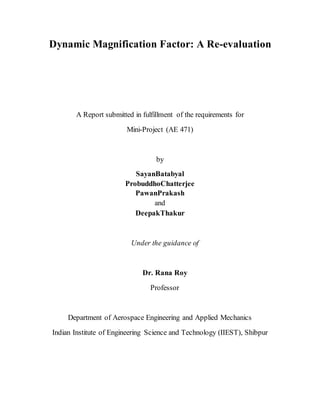
8.     222
0
21
1
nn
steady
k
F
x
DMF
 


………… (5)
Re-evaluationof Dynamic MagnificationFactor-
In order to recognize the significance of transient response on DMF over the traditional one, we
compute DMF at the exclusion 










k
F
x
DMF
steady
0
as well as inclusion 










k
F
x
DMF total
0
*
of the
transient response. Figure3 represents DMF and DMF* so computed for a range of β and ζ. This
indicates that the response may be marginally increased in the neighborhood of β=1. For ζ=0,
the range of frequency ratio that may lead to infinitely large response may also be widened.
However to notice another significant characteristic, we plot
DMF
DMF *
as a function of β in
Figure 4. This reveals that the DMF may be significantly underestimated with increase of β
(that appears to begin at β=1 as observed in Figure 3 when transient response is neglected).
This observation motivates us to examine how the velocity and acceleration parameters are
influenced due to the neglect of transient response. Plots for steady
total
x
x


and staedy
total
x
x


respectively in
Figure5 and Figure6 appear to indicate dramatic increase with increase of β.

9. In sum, the present investigation emphasizes on the significance of transient response to
calculate DMF especially at large values of β unless the damping is potentially large. A similar
observation has been found elsewhere (Gil Martin et al., 2011).
Conclusion-
From the review and introspection to results, it appears that the response considering the entire
solution (including transient portion) may vary significantly relative to conventional solution
(taking only the steady-state portion). This variation is not very significant for lower values of
β, however as β exceeds approximately to unity, the variation between the two solutions
becomes considerable. This indicates that if the forcing frequency is considerably greater than
the natural frequency of the system, we must take into consideration the transient solution so
that we do not perform the analysis erroneously.

10. Figures
Figure1: Simple SDOF Oscillator
Figure 2a: Variation of x/(Fo/k) over the duration of excitation function

11. Figure 2b: Variation of x/ {(Fo/k)*ω}over the duration of excitation function
funffunctfunctionfunction
Figure 2c: Variation of x/{(Fo/k)*ω2}over the duration of excitation function
funffunctfunctionfunction

12. 0.00
2.00
4.00
6.00
8.00
10.00
12.00
14.00
16.00
0.00 0.50 1.00 1.50 2.00 2.50 3.00 3.50
DMF&DMF*
ω/ωn
Figure 3: Plot of DMF*(= xtotal / (Fo/k)) as a function of ω/ωn for different ζ (0.0 – 1.0), DMF (= xsteady / (Fo/k)) has been
superimposed for comparison

13. 0.00
0.50
1.00
1.50
2.00
2.50
3.00
3.50
0.00 0.50 1.00 1.50 2.00 2.50 3.00 3.50
DMF*/DMF
ω/ωn

14. 0.00
1.00
2.00
3.00
4.00
5.00
6.00
7.00
8.00
9.00
10.00
0.00 0.50 1.00 1.50 2.00 2.50 3.00 3.50
ω/ωn
Figure 4b: Variation of 𝑥̇ 𝑡𝑜𝑡𝑎𝑙 relative to 𝑥̇ 𝑠𝑡𝑒𝑎𝑑𝑦 as a function of frequency ratio (ω/ωn) for different ζ (0.0 – 1.0)

15. 0.00
5.00
10.00
15.00
20.00
25.00
30.00
0.00 0.50 1.00 1.50 2.00 2.50 3.00 3.50
ω/ωn
Figure 4c: Variation of 𝑥̈ 𝑡𝑜𝑡𝑎𝑙 relative to 𝑥̈ 𝑠𝑡𝑒𝑎𝑑𝑦 as a function of frequency ratio (ω/ωn) for different ζ (0.0 – 1.0)

16. Appendix A
Mathematical Modelling and Solution of Forced Vibration-
The equation of motion has already been shown as (equation 1b)-
m
Fxxx nn 
2
2  
This is a double differential equation and hence has to be solved using the rules of the same. So
we need to find the complementary function first and then the particular integrand.
The complementary function may be conveniently expressed as-
))sin()cos(( 11 tBtAex t
CF
n

 
……… (A1)
where 2
1 1  
Now we try to calculate the particular integrand.
Let us assume
n
  and k
m
F
n
2
0

. So-
)sin(
])2()1[(
cos2sin)1(
22
2
0







tXx
tt
k
F
x
…………. (A2)
]))(2())(1[(
cos2sin))(1(
])2()[(
cos2sin)(
sin
])2()[(
2)(
sin
])2()[(
2)(
sin
2
1
sin
2
1
sin2
222
2
2
0
2222
22
0
2222
22
0
2222
22
0
22
0
22
0
022
nn
nn
n
nn
nn
nn
nn
nn
nn
nn
nn
nn
tt
m
F
x
tt
m
F
x
t
D
m
F
x
t
D
m
F
x
t
Dm
F
x
t
DDm
F
x
t
m
F
xDxxD


































17. where
]4)1[( 2222
0
 
 k
F
X and
)1(
2
tan 2





Thus the total solution can be completely written as:-
)sin())sin()cos(( 11 
 
tXtBtAex tn
……… (A3)
Where 2
1 1  
222
0
)2())(1( nn
k
F
X
 








 
2
1
)(1
2
tan
n
n




18. Appendix B
Solution of Forced Vibration in the presence of Initial Conditions-
The application of the solution of the forced vibration model requires application in the real
world, and that is possible only when the boundary conditions are known and hence the
constants can be determined.
As we already know the solution (equation A3)-
)sin())sin()cos(( 11 
 
tXtBtAex tn
Here the constants A and B are unknown and thus requires the boundary conditions to
determine their values.
At t=0, generally the displacement and velocity are taken to be 0 i.e. at rest. So-
0)0( x and 0)0( x
Putting x=0-
)sin(
0)sin(


XA
XA


We can also calculate –
)cos()sincos()cossin( 111111  
 
tXtBtAetBtAex t
n
t nn

…… (A4)
Putting 𝑥̇=0 –






























cossin
1
cossin
cos
0cos
2
11
11
1
X
B
XXB
XAB
XAB
n
n
n
Using these boundary conditions we obtain the solution of the transient part as-

19.   )cos(cossinsin1
1
)sin(cossin)cos(sin1
1
)sin(cossin
1
)cos(sin
11
2
2
2
2
11
2
2
1
2
1
































































te
X
tte
X
t
X
tXex
t
t
t
transient
n
n
n
where 2
22
2
1
12
21
sin1
cossin
tan













Thus the total solution under the boundary conditions has taken the form as-
  


























)sin()cos(cossinsin1
1
11
2
2
2
2






tt
e
Xx
tn
… (A5)
where 222
0
)2())(1( nn
k
F
X
 

2
22
2
1
12
21
sin1
cossin
tan













and 2
1
2
tan





These values have been extensively used in the text and in the graphs to obtain the results.

20. References
1. Luisa Maria Gil-Martin, Juan Francisco Carbonell-Marquez, Enrique Hernandez-Montes,
Mark Aschheim and M.Pasadas Fernandez, ‘Dynamic Magnification Factor of SDOF
Oscillators under harmonic loading’.
2. Clough, R.W. and Penzien, J. Dynamicsof Structures, 2nd Edition. McGraw-Hill. 1993
3. Chopra, A.K. Dynamics of Structures-Theory and Applications to Earthquake
Engineering, 3rd Edition. Prentice Hall
4. Singiresu S. Rao MechanicalVibrations, 5th Edition. Prentice Hall