Present Value Table (PV Factor) are enlisted here.

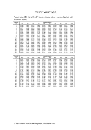
1. PRESENT VALUE TABLE
Present value of $1, that is  where r = interest rate; n = number of periods until
payment or receipt.
 n
r


1
Interest rates (r)
Periods
(n) 1% 2% 3% 4% 5% 6% 7% 8% 9% 10%
1 0.990 0.980 0.971 0.962 0.952 0.943 0.935 0.926 0.917 0.909
2 0.980 0.961 0.943 0.925 0.907 0.890 0.873 0.857 0.842 0.826
3 0.971 0.942 0.915 0.889 0.864 0.840 0.816 0.794 0.772 0.751
4 0.961 0.924 0.888 0.855 0.823 0.792 0.763 0.735 0.708 0.683
5 0.951 0.906 0.863 0.822 0.784 0.747 0.713 0.681 0.650 0.621
6 0.942 0.888 0.837 0.790 0.746 0705 0.666 0.630 0.596 0.564
7 0.933 0.871 0.813 0.760 0.711 0.665 0.623 0.583 0.547 0.513
8 0.923 0.853 0.789 0.731 0.677 0.627 0.582 0.540 0.502 0.467
9 0.914 0.837 0.766 0.703 0.645 0.592 0.544 0.500 0.460 0.424
10 0.905 0.820 0.744 0.676 0.614 0.558 0.508 0.463 0.422 0.386
11 0.896 0.804 0.722 0.650 0.585 0.527 0.475 0.429 0.388 0.350
12 0.887 0.788 0.701 0.625 0.557 0.497 0.444 0.397 0.356 0.319
13 0.879 0.773 0.681 0.601 0.530 0.469 0.415 0.368 0.326 0.290
14 0.870 0.758 0.661 0.577 0.505 0.442 0.388 0.340 0.299 0.263
15 0.861 0.743 0.642 0.555 0.481 0.417 0.362 0.315 0.275 0.239
16 0.853 0.728 0.623 0.534 0.458 0.394 0.339 0.292 0.252 0.218
17 0.844 0.714 0.605 0.513 0.436 0.371 0.317 0.270 0.231 0.198
18 0.836 0.700 0.587 0.494 0.416 0.350 0.296 0.250 0.212 0.180
19 0.828 0.686 0.570 0.475 0.396 0.331 0.277 0.232 0.194 0.164
20 0.820 0.673 0.554 0.456 0.377 0.312 0.258 0.215 0.178 0.149
Interest rates (r)
Periods
(n) 11% 12% 13% 14% 15% 16% 17% 18% 19% 20%
1 0.901 0.893 0.885 0.877 0.870 0.862 0.855 0.847 0.840 0.833
2 0.812 0.797 0.783 0.769 0.756 0.743 0.731 0.718 0.706 0.694
3 0.731 0.712 0.693 0.675 0.658 0.641 0.624 0.609 0.593 0.579
4 0.659 0.636 0.613 0.592 0.572 0.552 0.534 0.516 0.499 0.482
5 0.593 0.567 0.543 0.519 0.497 0.476 0.456 0.437 0.419 0.402
6 0.535 0.507 0.480 0.456 0.432 0.410 0.390 0.370 0.352 0.335
7 0.482 0.452 0.425 0.400 0.376 0.354 0.333 0.314 0.296 0.279
8 0.434 0.404 0.376 0.351 0.327 0.305 0.285 0.266 0.249 0.233
9 0.391 0.361 0.333 0.308 0.284 0.263 0.243 0.225 0.209 0.194
10 0.352 0.322 0.295 0.270 0.247 0.227 0.208 0.191 0.176 0.162
11 0.317 0.287 0.261 0.237 0.215 0.195 0.178 0.162 0.148 0.135
12 0.286 0.257 0.231 0.208 0.187 0.168 0.152 0.137 0.124 0.112
13 0.258 0.229 0.204 0.182 0.163 0.145 0.130 0.116 0.104 0.093
14 0.232 0.205 0.181 0.160 0.141 0.125 0.111 0.099 0.088 0.078
15 0.209 0.183 0.160 0.140 0.123 0.108 0.095 0.084 0.079 0.065
16 0.188 0.163 0.141 0.123 0.107 0.093 0.081 0.071 0.062 0.054
17 0.170 0.146 0.125 0.108 0.093 0.080 0.069 0.060 0.052 0.045
18 0.153 0.130 0.111 0.095 0.081 0.069 0.059 0.051 0.044 0.038
19 0.138 0.116 0.098 0.083 0.070 0.060 0.051 0.043 0.037 0.031
20 0.124 0.104 0.087 0.073 0.061 0.051 0.043 0.037 0.031 0.026
 The Chartered Institute of Management Accountants 2010

2. Cumulative present value of $1 per annum, Receivable or Payable at the end of each year for n
years r
r n


 )
(1
1
Interest rates (r)
Periods
(n) 1% 2% 3% 4% 5% 6% 7% 8% 9% 10%
1 0.990 0.980 0.971 0.962 0.952 0.943 0.935 0.926 0.917 0.909
2 1.970 1.942 1.913 1.886 1.859 1.833 1.808 1.783 1.759 1.736
3 2.941 2.884 2.829 2.775 2.723 2.673 2.624 2.577 2.531 2.487
4 3.902 3.808 3.717 3.630 3.546 3.465 3.387 3.312 3.240 3.170
5 4.853 4.713 4.580 4.452 4.329 4.212 4.100 3.993 3.890 3.791
6 5.795 5.601 5.417 5.242 5.076 4.917 4.767 4.623 4.486 4.355
7 6.728 6.472 6.230 6.002 5.786 5.582 5.389 5.206 5.033 4.868
8 7.652 7.325 7.020 6.733 6.463 6.210 5.971 5.747 5.535 5.335
9 8.566 8.162 7.786 7.435 7.108 6.802 6.515 6.247 5.995 5.759
10 9.471 8.983 8.530 8.111 7.722 7.360 7.024 6.710 6.418 6.145
11 10.368 9.787 9.253 8.760 8.306 7.887 7.499 7.139 6.805 6.495
12 11.255 10.575 9.954 9.385 8.863 8.384 7.943 7.536 7.161 6.814
13 12.134 11.348 10.635 9.986 9.394 8.853 8.358 7.904 7.487 7.103
14 13.004 12.106 11.296 10.563 9.899 9.295 8.745 8.244 7.786 7.367
15 13.865 12.849 11.938 11.118 10.380 9.712 9.108 8.559 8.061 7.606
16 14.718 13.578 12.561 11.652 10.838 10.106 9.447 8.851 8.313 7.824
17 15.562 14.292 13.166 12.166 11.274 10.477 9.763 9.122 8.544 8.022
18 16.398 14.992 13.754 12.659 11.690 10.828 10.059 9.372 8.756 8.201
19 17.226 15.679 14.324 13.134 12.085 11.158 10.336 9.604 8.950 8.365
20 18.046 16.351 14.878 13.590 12.462 11.470 10.594 9.818 9.129 8.514
Interest rates (r)
Periods
(n) 11% 12% 13% 14% 15% 16% 17% 18% 19% 20%
1 0.901 0.893 0.885 0.877 0.870 0.862 0.855 0.847 0.840 0.833
2 1.713 1.690 1.668 1.647 1.626 1.605 1.585 1.566 1.547 1.528
3 2.444 2.402 2.361 2.322 2.283 2.246 2.210 2.174 2.140 2.106
4 3.102 3.037 2.974 2.914 2.855 2.798 2.743 2.690 2.639 2.589
5 3.696 3.605 3.517 3.433 3.352 3.274 3.199 3.127 3.058 2.991
6 4.231 4.111 3.998 3.889 3.784 3.685 3.589 3.498 3.410 3.326
7 4.712 4.564 4.423 4.288 4.160 4.039 3.922 3.812 3.706 3.605
8 5.146 4.968 4.799 4.639 4.487 4.344 4.207 4.078 3.954 3.837
9 5.537 5.328 5.132 4.946 4.772 4.607 4.451 4.303 4.163 4.031
10 5.889 5.650 5.426 5.216 5.019 4.833 4.659 4.494 4.339 4.192
11 6.207 5.938 5.687 5.453 5.234 5.029 4.836 4.656 4.486 4.327
12 6.492 6.194 5.918 5.660 5.421 5.197 4.988 7.793 4.611 4.439
13 6.750 6.424 6.122 5.842 5.583 5.342 5.118 4.910 4.715 4.533
14 6.982 6.628 6.302 6.002 5.724 5.468 5.229 5.008 4.802 4.611
15 7.191 6.811 6.462 6.142 5.847 5.575 5.324 5.092 4.876 4.675
16 7.379 6.974 6.604 6.265 5.954 5.668 5.405 5.162 4.938 4.730
17 7.549 7.120 6.729 6.373 6.047 5.749 5.475 5.222 4.990 4.775
18 7.702 7.250 6.840 6.467 6.128 5.818 5.534 5.273 5.033 4.812
19 7.839 7.366 6.938 6.550 6.198 5.877 5.584 5.316 5.070 4.843
20 7.963 7.469 7.025 6.623 6.259 5.929 5.628 5.353 5.101 4.870
May 2010 2 Performance Operations

3. FORMULAE
PROBABILITY
A B = A or B. A B = A and B (overlap).
 
P(B A) = probability of B, given A.
Rules of Addition
If A and B are mutually exclusive: P(A  B) = P(A) + P(B)
If A and B are not mutually exclusive: P(A B) = P(A) + P(B) – P(A
  B)
Rules of Multiplication
If A and B are independent: P(A B) = P(A) * P(B)

If A and B are not independent: P(A  B) = P(A) * P(B | A)
E(X) = (probability * payoff)

DESCRIPTIVE STATISTICS
Arithmetic Mean
n
x
x


f
fx
x


 (frequency distribution)
Standard Deviation
n
x
x
SD
2
)
( 

 2
2
x
f
fx
SD 


 (frequency distribution)
INDEX NUMBERS
Price relative = 100 * P1/P0 Quantity relative = 100 * Q1/Q0
Price: 100
x
w
P
P
w
o
1











Quantity: 100
x
1
w
Q
Q
w
o











TIME SERIES
Additive Model
Series = Trend + Seasonal + Random
Multiplicative Model
Series = Trend * Seasonal * Random
May 2010 3 Performance Operations

4. FINANCIAL MATHEMATICS
Compound Interest (Values and Sums)
Future Value S, of a sum of X, invested for n periods, compounded at r% interest
S = X[1 + r]n
Annuity
Present value of an annuity of £1 per annum receivable or payable for n years, commencing in one
year, discounted at r% per annum:
PV =









 n
r
r ]
1
[
1
1
1
Perpetuity
Present value of £1 per annum, payable or receivable in perpetuity, commencing in one year,
discounted at r% per annum:
PV =
r
1
LEARNING CURVE
Yx = aX
b
where:
Yx = the cumulative average time per unit to produce X units;
a = the time required to produce the first unit of output;
X = the cumulative number of units;
b = the index of learning.
The exponent b is defined as the log of the learning curve improvement rate divided by log 2.
INVENTORY MANAGEMENT
Economic Order Quantity
EOQ =
h
o
C
D
2C
where: Co = cost of placing an order
Ch = cost of holding one unit in Inventory for one year
D = annual demand
May 2010 4 Performance Operations