F-302 Managerial Accounting

of 142
Table of Contents
Chapter One: Introduction.....................................................................................................4
1.1 Origin of the Report.........................................................................................................4
1.2 Objective of the Report....................................................................................................5
1.3 Scope of the Report..........................................................................................................6
1.4 Limitations of the Report.................................................................................................7
1.5 Sources and Methodology................................................................................................8
Chapter Two: Overview of Company....................................................................................9
2.1 History of the Glaxo SmithKline limited.........................................................................9
2.2 Corporate highlights of Glaxo SmithKline....................................................................11
2.3 Mission of Glaxo SmithKline........................................................................................12
2.4 Strategy of Glaxo SmithKline........................................................................................13
2.5 Values of Glaxo SmithKline..........................................................................................15
2.6 Products of Glaxo SmithKline.......................................................................................16
2.7 Responsibilities of Glaxo SmithKline ...........................................................................18
2.8 Organizational structure of Glaxo SmithKline ..............................................................19
2.9 Shareholder’s information of Glaxo SmithKline...........................................................20
Chapter Three: Theoretical Background............................................................................23
3.1 Managerial Accounting:.................................................................................................23
3.2 Importance of managerial accounting .......................................................................23
3.3 Comparison between managerial and financial accounting...........................................25
3.4 General cost classification .............................................................................................26
3.5 Product Costs versus Period Costs:................................................................................29
3.5 Cost Classifications on Financial Statements: ...............................................................30
3.6 Cost Classifications for Predicting Cost Behavior: .......................................................32
3.8 Cost Classifications for Assigning Costs to Cost Objects:............................................33
3.9 Cost Classifications for Decision Making: ....................................................................35
Chapter Four: Implication of managerial accounting and cost concept on Glaxo
SmithKline..............................................................................................................................37
4.1 Cost classification of Glaxo SmithKline........................................................................37
4.2 Calculation of Cost of goods sold of Glaxo SmithKline for different years .................39
4.3 Graphical presentation of CGS and net operating of Glaxo SmithKline.......................41
Chapter Five: Cost-volume Profit analysis of Glaxo SmithKline .....................................43

of 142
5.1 Fundamental concept of Cost – Volume – Profit Analysis: ..........................................43
5.1.1 Overview of Cost-Volume Profit Analysis:............................................................44
5.1.2 CVP Relationships in Equation Form:....................................................................47
5.1.3 CVP Relationships in Graphic Form: .....................................................................48
5.1.4 Contribution Margin Ratio (CM Ratio):.................................................................50
5.2 Implication of CVP analysis on Glaxo SmithKline.......................................................55
Chapter Six: Variable Costing Analysis ..............................................................................62
6.1 Fundamental concept of variable costing ......................................................................62
6.2 Implication of variable costing concept on Glaxo SmithKline......................................64
6.3 Comparative Income Effects—Absorption and Variable Costing.................................68
6.4 Comparative Advantages of Variable costing: ..............................................................69
Chapter Seven: Activity based Costing Analysis................................................................70
7.1 Fundamental concept of activity based costing .............................................................70
Activity Based Costing: An overview:..............................................................................70
7.2 Implication of activity based costing on Glaxo SmithKline..........................................78
Chapter Eight: Profit planning.............................................................................................91
8.1 Fundamental concept of profit planning........................................................................91
8.2 Implication of profit planning concept on Glaxo SmithKline .......................................99
Chapter Nine: Flexible budget and performance analysis...............................................105
9.1 Fundamental concept of Flexible budget and performance analysis...........................105
9.2 Implication of flexible budget and performance analysis on Glaxo SmithKline.........109
Chapter Ten: Standards cost and operating performance measures .............................113
10.1 Fundamental concept of Standard cost and operating performance measures ..........113
10.2 Implication of fundamental concept of standard cost and operating performance
measures on Glaxo SmithKline .........................................................................................117
Chapter Eleven: Segmented Reporting, Decentralization, and the Balanced Scorecard
................................................................................................................................................128
11.1 Fundamental concept of Segmented Reporting, Decentralization, and the Balanced
Scorecard............................................................................................................................128
11.2 Implication of Segmented Reporting, Decentralization, and the Balanced Scorecard
............................................................................................................................................130
Chapter Twelve: Suggestion and Conclusion....................................................................140
12.1 Suggestions:...............................................................................................................140
12.2 Conclusion .................................................................................................................141

of 142
Reference ..............................................................................................................................142
References...........................................................................Error! Bookmark not defined.

of 142
Chapter One: Introduction
1.1 Origin of the Report
To have an overview of Managerial Accounting in practical life we’ve a study on Glaxo
SmithKline Company, a drug manufacturer company and one of the largest companies in
the world. Now a day’s education is not just limited to books and classrooms. In today’s
world, education is the tool to understand the real world and apply knowledge for the
betterment of the society as well as business. From education the theoretical knowledge is
obtained from courses of study, which is only the half way of the subject matter. Practical
knowledge has no alternative. The perfect coordination between theory and practice is of
paramount importance in the context of the modern business world in order to resolve the
dichotomy between these two areas. Therefore, for the B.B.A. program we are assigned to
prepare a report on “Glaxo SmithKline” for Managerial Accounting (F-302) course by our
honorable course teachers Md. Imran Hossain and Sultana Shahreen Karim.

of 142
1.2 Objective of the Report
Our objectives are……….
 To increase our experience in data collection & analysis.
 To know about the actual picture of Glaxo SmithKline.
 To have practical knowledge of Managerial accounting.
 To know the implications of Managerial accounting on Glaxo SmithKline.
 To have better analytical abilities regarding managerial accounting in rea
world.
 To know Glaxo SmithKline from a closer view.

of 142
1.3 Scope of the Report
While completing the report we’ve had a lot of scopes of gathering knowledge of real
business world and the wide horizon of business, although the report is only concerned
about the Glaxo SmithKline Company. We have collected their information from the
internet as it a multinational company and its head office is outside of Bangladesh. We got
almost all the information we needed because the website of the company is very much
updated and resourceful. We knew about their mission, vision, products, area of operation,
accounting system, managerial and organizational structure etc. We are really grateful to
our course teachers for assigning us such an interesting and knowledgeable topic.

of 142
1.4 Limitations of the Report
While preparing this report, we have faced some problems. The main problem was to co-
ordination all the group members. Moreover, during data collection we faced several
problems.
 Due to limited access of the data, this study may not be perfect to the scent percent.
 Lack of enough experience in analyzing of data.
 Due to inadequate information, in-depth analysis could not be done in the report.

of 142
1.5 Sources and Methodology
This report’s research is based on application of managerial accounting in Glaxo
SmithKline Company. The data types are secondary that were collected from the internet.
The company’s updated information is given on its website and we mainly collected
information from there.
Sources of information:
Company’s published annual report.
Analysis about the company by others.
Company’s websites.

of 142
Chapter Two: Overview of Company
2.1 History of the Glaxo SmithKline limited
GlaxoSmithKline (GSK) was created in 2001 in the merger of two established companies,
Glaxo Wellcome and SmithKline Beecham. These companies originated in the United
States and England, respectively, and their histories include a series of mergers that began
in the 1800s. Glaxo Wellcome was created in 1995 when Jason Nathan and Company,
started in 1873, merged with Burroughs Wellcome and Company, started by Henry
Wellcome and Silas Burroughs in 1880. SmithKline Beecham began with John K. Smith
opening a drugstore in Philadelphia in 1830. He was joined by Mahlon Kline in 1865.
Together Smith and Kline acquired numerous companies, like a vaccines business and,
most notably, French Richards and Company, another well-respected drug wholesaler.
Meanwhile, Thomas Beecham began his Beecham’s Pills business in England in 1842. One
of Beecham’s first products, a laxative made from aloe, ginger and soap, became very
successful. Later, scientists from the company’s research laboratory discovered amoxicillin
and sold the antibiotic as Amoxil in 1972. Amoxil was widely accepted. Beecham merged
with Smith and Kline in 1989 to become SmithKlineBeecham.

of 142
The merger of Glaxo Wellcome and SmithKline Beecham created GlaxoSmithKline in
2001. Today the company is divided into three main segments: pharmaceuticals (treating
cancer, heart disease and HIV/AIDs), vaccines (treating hepatitis, polio and typhoid), and
consumer health care (treating oral and skin problems) and has grown steadily, selling
products in more than 170 countries.
GSK partners with the World Health Organization (WHO), seeking to fight lymphatic
filariasis (intestinal worms). In 2002, the company donated 100 million albendazole
tablets to treat the condition. It also established one of the largest vaccine businesses in
the world, distributing more than 1.1 billion doses of its vaccines to 173 countries. More
recently, GSK set itself apart by receiving approval for the first new lupus treatment in
50 years and by providing laboratory equipment for the 2012 Olympics.

of 142
2.2 Corporate highlights of Glaxo SmithKline
Name of the Company Glaxo SmithKline
Founded in 2000
Type Public Limited Company
Treaded as LSE: GSK
NYSE:GSK
Industry Pharmaceutical
Biotechnology
Consumer goods
Predecessors Glaxo Wellcome and SmithKline Beecham
Headquarters Brentford, London
Key people Sir Philip Hampton (Chairman)
Andrew Witty (CEO)
Products Pharmaceuticals, vaccines, oral, healthcare,
nutritional products, over-the-counter medicines.
Revenue 23.923 billion pound (2015)
Operating Income 10.322 billion pound (2015)
Net Income 8.372 billion pound (2015)
Number of employees 96575 (2015)
Subsidiaries Stiefel Laboratories
Slogan “Do more, feel better, live longer”
Website www.gsk.com

of 142
2.3 Mission of Glaxo SmithKline
Mission is defined as an important assignment carried out for political, religious, or
commercial purposes. In another way mission is strongly felt aim, ambition, or calling. All
most everyone or every entity has mission. The company organization’s missions are stated
in company’s “Mission Statement”. Let’s know about the mission of Glaxo SmithKline
Company.
Glaxo SmithKline Company’s mission is to “improve the quality of human life
by enabling people to do more, feel better and live longer.”

of 142
2.4 Strategy of Glaxo SmithKline
Strategy is the direction and scope of an organization over the long-term: which achieves
advantage for the organization through its configuration of resources within a challenging
environment, to meet the needs of markets and to fulfill stakeholder expectations".
In other words, strategy is about:
 Where is the business trying to get to in the long-term (direction?)
 Which markets should a business compete in and what kind of activities is involved in
such markets? (Markets; scope)
 How can the business perform better than the competition in those markets?
(Advantage)
 What resources (skills, assets, finance, relationships, technical competence, and
facilities) are required in order to be able to compete? (Resources)
 What external, environmental factors affect the businesses' ability to compete?
(Environment)
 What are the values and expectations of those who have power in and around the
business? (Stakeholders)
Strategy at Different Levels of a Business Strategies exists at several levels in any
organization - ranging from the overall business (or group of businesses) through to
individuals working in it.

of 142
Corporate Strategy - is concerned with the overall purpose and scope of the business to
meet stakeholder expectations. This is a crucial level since it is heavily influenced by
investors in the business and acts to guide strategic decision- making throughout the
business.
Strategies of Glaxo SmithKline are:
 Grow a diversified global company.
 Deliver more products of value.
 Simplify the operating model.
 Individual empowerment.
 Build trust.
In practice, a thorough strategic management process has three main components, shown in the
figure below:
Strategic
Analysis
Strategy
implementation
Strategic
choice

of 142
2.5 Values of Glaxo SmithKline
Values are the belief about what is right and what is wrong, what we should we do, and
what we should not. In business organizations, there always prevail values. Some
organizations give much important to these values because values represent an organization
in outside the organization. In Glaxo SmithKline Company, we found there stated values.
These are;
values
Respect for
People
Patient Focus
Transparency
Integrity

of 142
2.6 Products of Glaxo SmithKline

of 142
Products sold by Glaxo SmithKline
Drug
Augmentin
Serevent
Avandia
Wellutrin
Lamictal
Zofran
Vaccines
Cervavix
MeHibrix
Fluarix Quadrivalent
Pediarix
FluLaval
Typherix
Healthcare Items
Aquafresh Breathe Right Sebsodyne

of 142
2.7 Responsibilities of Glaxo SmithKline
Responsibilities are the duties required to be done. Business responsibilities are often
called Corporate Social Responsibilities. Responsibilities should be done simultaneously
and responsible business organizations become successful in all most every step of
business arena.
At Glaxo SmithKline (GSK) responsible business is how they do business. Their mission
is to improve quality of human life by enabling people to do more, feel better, live longer.
Responsibilities of GSK are given bellow;
Commitments
• Ensuring health for
all
• Noble behaviour
• Employee protection
• Environmental
activities
Oversight
• Corporate Social
Activities supportive
organizatonal
structure.
Shareholders
protecton
• More interaction
with them.
• Working for their
highest benefit

of 142
2.8 Organizational structure of Glaxo SmithKline
In GSK, They have a robust governance structure in place to evaluate our policies and
programmers, and ensure the approach we take on corporate responsibility issues is
appropriate. Our board-level Corporate Responsibility Committee (CRC) has overall
responsibility and sits within a clear organizational structure that ensures accountability.
Figure 1: Organizational Structure of Glaxo SmithKline
Board
(Chairman, 3 Executive
Directors and 11 independent
Non-Executive Directors)
Audit and Risk
Committee
Corporate
Responsibility
Committee
Remuneration
Committee
Finance
Committee
Nominations
Committee
Corporate
Administration
and Transactions
Committee
Chief Executive
Office
Corporate
Executive
Team

of 142
2.9 Shareholder’s information of Glaxo SmithKline
Glaxo SmithKline has a strong shareholding position in the market compared to other
competitors. The volumes of shares are very healthy and productive that is owned by different
types of shareholders. It shows shareholdings are diversified as well. Now we present
shareholding position of Glaxo SmithKline from the year 2010 to 2014.
Figure 2: Shareholding position of 2010
81.98%
12.09%
4.06% 1.87%
Shareholding position of 2010
Share holding position of 2010 Parent company
ICB General Public
Other financial institutions
81.98%
12.01%
4.58% 1.43%
ICB General Public

of 142
81.98%
12.10%
3.70% 2.22%
ICB General Public
81.98%
12.10%
3.70% 2.22%
ICB General Public

of 142
ICB General Public

of 142
Chapter Three: Theoretical Background
3.1 Managerial Accounting:
Managerial accounting is concerned with providing information to managers—that is, the
people inside an organization who direct and control its operations. According to the Institute
of Management Accountants (IMA): "Management accounting is a profession that involves
partnering in management decision making, devising planning and performance management
systems, and providing expertise in financial reporting and control to assist management in the
formulation and implementation of an organization's strategy".
3.2 Importance of managerial accounting
The main Advantage of management accounting is given below:
Determination of Aim: Management accounting on the basis of the information
available determines its goal and tries to find out the route through which it can reach
the goal.
Helps in the Preparation of Plan: Present age is the age of planning. That producer is
considered as most successful producer who produces articles according to the plan and
needs of the consumers. Before taking any plan the manager must study and analyze
the present and future of the business.
Better Services to Customers: The cost control device is management accounting
enables the reduction in prices of the Product. All employees in the concern are made
cost Conesus. The quality of the Product become well because quality standards ate
pre-determined. The Customers are supplied goods and goods quality at reasonable
price.
Easy to take judgment: Before taking any plan or to determine policy. There are several
plans or policies before the management on the basis of the study he decides which plan
and policy was to be adapted so that it may be more useful and helpful.
Measurements of performance: The techniques of budgetary control standard costing
enables the measurement of performance In standard costing, standards are determined

of 142
1st
and then actual cost of compared with standard cost. It enables the management to
find out deviations between standard cost and actual cost. The performance will be good
it actual cost does not exceed the standard cost. Budgetary control system too helps in
measuring efficiency of all employees.
Increase Efficiency of the business: Management accounting increases efficiency of
the business concern. The targets of different departments of the enterprise are
determined in advance and the achievement of these goals is taken as a tool for
measuring their efficiency.
Provide effective management control: The Tools and techniques of the management
accounting are helpful to the management in planning controlling and coordinating
activities of the business, the getting of standard and assessing actual performance
regularly enables the management to have ‘management by exception’. Everybody
assesses his own work and immediate actions are taken as a tool for measuring their
efficiency.
Maximum profits of can be obtained: In this process every possible effort are made to
control unnecessary expenses. The incapability or inefficiency is removed. New
systems or techniques are found out to achieve the goal, so that there may be maximum
profits out if the capital invested in the Business.
Safety and security from trade cycle: The Information received from the management
accounting gives more or throws enough light over the past trade cycle. The
management tries to ascertain the Causes of trade cycle and its affect. Thus,
management accounting tries to safeguard the organization from the effect of trade
cycle.

of 142
3.3 Comparison between managerial and financial accounting
Managerial accounting is concerned with providing information to managers—that is, the
people inside an organization who direct and control its operations. In contrast, financial
accounting is concerned with providing information to stockholders, creditors, and others
who are outside the organization. This contrast in orientation, results in a number of major
differences between financial and managerial accounting, even though they often rely on the
same underlying financial data.
Subject of
Difference
Financial Accounting Managerial Accounting
1.Meaning Financial Accounting is an
accounting system that focuses on
the preparation of financial
statement of an organization to
provide the financial information
to the interested parties
The accounting system which
provides relevant information to
the managers to make policies,
plans and strategies for running
the business effectively is
known as Management
Accounting.
2. User Internal and external parties. Only internal management.
3.Time
Frame
Financial Statements are prepared
at the end of the accounting period
which is usually one year.
The reports are prepared as per
the need and requirements of the
organization.
4.Objective To provide financial information
to outsiders.
To assist the management in
planning and decision making
process by providing detailed
information on various matters.
5.Efficiency Financial accounting reports on
the profitability (and therefore the
efficiency) of a business.
Whereas managerial accounting
reports on specifically what is
causing problems and how to fix
them.
6. Format Specified Not specified
7. Reports Summarized Reports about the
financial position of the
organization
Complete and Detailed reports
regarding various information.

of 142
3.4 General cost classification
We have chosen to start our discussion of cost concepts by focusing on manufacturing
companies, because they are involved in most of the activities found in other types of
organizations.
1. Manufacturing Costs: Most manufacturing companies separate manufacturing costs into
three broad categories: direct materials, direct labor, and manufacturing overhead. A
discussion of each of these categories follows.
Figure 7: Classification of Manufacturing Cost
i. Direct Materials: The materials that go into the final product are called raw materials.
This term is somewhat misleading because it seems to imply unprocessed natural resources
like wood pulp or iron ore. Actually, raw materials refer to any materials that are used in
the final product; and the finished product of one company can become the raw materials
of another company.
Raw materials may include both direct and indirect materials. Direct materials are those
materials that become an integral part of the finished product and whose costs can be
Manufacturing
Cost
Direct
Materials
Direct Labor
Manufacturing
overhead
Prime Cost
Conversion
Cost

of 142
conveniently traced to the finished product. This would include, for example, the seats that
Airbus purchases from subcontractors to install in its commercial aircraft and the tiny
electric motor Panasonic uses in its DVD players. Materials such as solder and glue are
called indirect materials and are included as part of manufacturing overhead, which is
discussed later in this section.
ii. Direct Labor: Direct Labor consists of labor costs that can be easily (i.e., physically
and conveniently) traced to individual units of product. Direct labor is sometimes called
touch labor because direct labor workers typically touch the product while it is being
made. Examples of direct labor include assembly-line workers at Toyota, carpenters at the
home builder Kaufman and Broad, and electricians who install equipment on aircraft at
Bombardier Learjet.
Labor costs that cannot be physically traced to particular products, or that can be traced
only at great cost and inconvenience, are termed indirect labor. Just like indirect
materials, indirect labor is treated as part of manufacturing overhead. Indirect labor
includes the labor costs of janitors, supervisors, materials handlers, and night security
guards. Although the efforts of these workers are essential, it would be either impractical
or impossible to accurately trace their costs to specific units of product. Hence, such labor
costs are treated as indirect labor.
iii. Manufacturing Overhead: Manufacturing overhead, the third element of
manufacturing cost, includes all manufacturing costs except direct materials and direct
labor. Manufacturing overhead includes items such as indirect materials; indirect labor;
maintenance and repairs on production equipment; and heat and light, property taxes,
depreciation, and insurance on manufacturing facilities. A company also incurs costs for
heat and light, property taxes, insurance, depreciation, and so forth, associated with its
selling and administrative functions, but these costs are not included as part of
manufacturing overhead. Only those costs associated with operating the factory are
included in manufacturing overhead.

of 142
2. Nonmanufacturing Costs: Nonmanufacturing costs are often divided into two
categories: selling costs and administrative costs.
Figure 8: Non-Manufacturing Cost
i. Selling costs: Selling costs include all costs that are incurred to secure customer orders
and get the finished product to the customer. These costs are sometimes called order-
getting and order-filling costs. Examples of selling costs include advertising, shipping,
sales travel, sales commissions, sales salaries, and costs of finished goods warehouses.
ii. Administrative costs: Administrative costs include all costs associated with the general
management of an organization rather than with manufacturing or selling. Examples of
administrative costs include executive compensation, general accounting, secretarial,
public relations, and similar costs involved in the overall, general administration of the
organization as a whole.
Prime Cost and Conversion Cost:
Two more cost categories are often used in discussions of manufacturing costs— prime
cost and conversion cost. Prime cost is the sum of direct materials cost and direct labor
cost. Conversion cost is the sum of direct labor cost and manufacturing overhead cost.
The term conversion cost is used to describe direct labor and manufacturing overhead
because these costs are incurred to convert materials into the finished product.
Non-
Manufacturing
Cost
Selling Cost
Administrative
Cost

of 142
3.5 Product Costs versus Period Costs:
In addition to classifying costs as manufacturing or nonmanufacturing costs, there are other
ways to look at costs. For instance, they can also be classified as either product costs or period
costs.
Product Costs Period Costs
Product costs include all costs involved in
acquiring or making a product
Period costs are all the costs that are not product
costs.
Product costs consist of direct materials, direct
labor, and manufacturing overhead.
All selling and administrative expenses are
considered to be period costs
Product costs are initially assigned to
inventories; they are also known as inventor
able costs.
Period costs are not initially assigned to
inventories.
Direct and indirect raw material, labor costs,
etc.
Advertising, executive salaries, sales
commissions, public relations, another
nonmanufacturing costs discussed earlier are all
examples of period costs.

of 142
3.6 Cost Classifications on Financial Statements:
In this section of the chapter, we compare the cost classifications used on the financial
statements of manufacturing and merchandising companies. The financial statements
prepared by a manufacturing company are more complex than the statements prepared by
a merchandising company because a manufacturing company must produce its goods as
well as market them.
1. The Balance Sheet:
The balance sheet, or statement of financial position, of a manufacturing company is similar
to that of a merchandising company. However, their inventory accounts differ. A
merchandising company has only one class of inventory—goods purchased from suppliers
for resale to customers. In contrast, manufacturing companies have three classes of
inventories— raw materials, work in process, and finished goods. Raw materials are the
materials that are used to make a product. Work in process consists of units of product
that are only partially complete and will require further work before they are ready for sale
to a customer. Finished goods consist of completed units of product that have not yet been
sold to customers. Ordinarily, the sum total of these three categories of inventories is the
only amount shown on the balance sheet in external reports. However, the footnotes to the
financial statements often provide more detail.
Costs
Selling and administrative
cost
Raw materials
purchased
Direct Labor
Manufacturing
overhead
Balance Sheet
Raw materials inventory
Work in process
inventory
Finished goods
inventory
Income statement
Cost of goods sold
Selling and
administrative cost
Figure 9: Cost classification based on financial statements

of 142
2. The Income Statement:
The income statements of merchandising and manufacturing companies like Reston
Bookstore and Graham Manufacturing are very similar. The only apparent difference is
in the labels of some of the entries in the computation of the cost of goods sold.
Basic Equation for Inventory Accounts:
Beginning Balance + Addition to I inventory = Ending balance + Withdrawals from
inventory
The beginning inventory consists of any units that are in the inventory at the beginning
of the period. Additions are made to the inventory during the period. The sum of the
beginning balance and the additions to the account is the total amount of inventory
available. During the period, withdrawals are made from inventory. The ending balance
is whatever is left at the end of the period after the withdrawals.
Cost of Goods Sold in a Merchandising Company:
Cost of goods sold = Beginning merchandise inventory + Purchases – Ending
merchandise inventory
Cost of Goods Sold in a Manufacturing Company:
Cost of goods sold* = Beginning finished goods inventory + Cost of goods manufactured
- Ending finished goods inventory
3. Schedule of Cost of Goods Manufactured:
The schedule of cost of goods manufactured contains the three elements of product costs
that we discussed earlier—direct materials, direct labor, and manufacturing overhead.
The subtle distinction between the total manufacturing cost and the cost of goods
manufactured is very easy to miss. Some of the materials, direct labor, and manufacturing
overhead. Costs incurred during the period relate to goods that are not yet completed. As
stated above, the cost of goods manufactured consists of the manufacturing costs
associated with the goods that were finished during the period. Consequently,
adjustments need to be made to the total manufacturing cost of the period for the partially
completed goods that were in process at the beginning and at the end of the period. The
costs that relate to goods that are not yet completed are shown in the work in process

of 142
inventory figures at the bottom of the schedule. Note that the beginning work in process
inventory must be added to the manufacturing costs of the period, and the ending work
in process inventory must be deducted, to arrive at the cost of goods manufactured.
Specimen of Schedule of Cost of Goods Manufactured
3.7 Cost Classifications for Predicting Cost Behavior:
Cost behavior refers to how a cost reacts to changes in the level of activity. As the activity
level rises and falls, a particular cost may rise and fall as well—or it may remain constant.
For planning purposes, a manager must be able to anticipate which of these will happen;
and if a cost can be expected to change, the manager must be able to estimate how much it
will change. To help make such distinctions, costs are often categorized as variable or fixed.
1. Variable Cost:
A variable cost is a cost that varies, in total, in direct proportion to changes in the level of
activity. The activity can be expressed in many ways, such as units produced, units sold,
miles driven, beds occupied, lines of print, hours worked, and so forth. A good example of
a variable cost is direct materials. The cost of direct materials used during a period will
vary, in total, in direct proportion to the number of units that are produced.

of 142
2. Fixed Cost:
A fixed cost is a cost that remains constant, in total, regardless of changes in the level of
activity. Unlike variable costs, fixed costs are not affected by changes in activity.
Consequently, as the activity level rises and falls, total fixed costs remain constant unless
influenced by some outside force, such as a price change. Rent is a good example of a
fixed cost.
3.8 Cost Classifications for Assigning Costs to Cost Objects:
Costs are assigned to cost objects for a variety of purposes including pricing, preparing
profitability studies, and controlling spending. A cost object is anything for which cost
data are desired—including products, customers, jobs, and organizational subunits. For
purposes of assigning costs to cost objects, costs are classified as either direct or indirect.
0
750500250
20,00
00
0
250 1000500
Uni
Co
Production in unit
Costs
30,000
20,000
10,000
Figure 10: Variable cost
Figure 11: Fixed cost

of 142
1. Direct Cost: A direct cost is a cost that can be easily and conveniently traced to a
specified cost object. The concept of direct cost extends beyond just direct materials and
direct labor. For example, if Reebok is assigning costs to its various regional and national
sales offices, then the salary of the sales manager in its Tokyo office would be a direct cost
of that office.
2. Indirect Cost: An indirect cost is a cost that cannot be easily and conveniently traced
to a specified cost object. For example, a Campbell Soup factory may produce dozens of
varieties of canned soups. The factory manager’s salary would be an indirect cost of a
particular variety such as chicken noodle soup. The reason is that the factory manager’s
salary is incurred as a consequence of running the entire factory—it is not incurred to
produce any one soup variety.
A particular cost may be direct or indirect, depending on the cost object. While the
Campbell Soup factory manager’s salary is an indirect cost of manufacturing chicken
noodle soup, it is a direct cost of the manufacturing division. In the first case, the cost
object is chicken noodle soup. In the second case, the cost object is the entire
manufacturing division.

of 142
3.9 Cost Classifications for Decision Making:
Costs are an important feature of many business decisions. In making decisions, it is
essential to have a firm grasp of the concepts differential cost, opportunity cost, and sunk
cost.
`
Figure 12: Cost classification based on decision making
1. Differential Cost and Revenue: A difference in costs between any two alternatives is
known as a differential cost. A difference in revenues between any two alternatives is
known as differential revenue. A differential cost is also known as an incremental cost
, although technically an incremental cost should refer only to an increase in cost from
one alternative to another; decreases in cost should be referred to as decremented costs.
Differential cost is a broader term, encompassing both cost increases (incremental costs)
and cost decreases (decremented costs) between alternatives.
2. Opportunity Cost: Opportunity cost is the potential benefit that is given up when
one alternative is selected over another. To illustrate this important concept, consider the
following examples: Vicki has a part-time job that pays $200 per week while attending
college. She would like to spend a week at the beach during spring break, and her
employer has agreed to give her the time off, but without pay. The $200 in lost wages
would be an opportunity cost of taking the week off to be at the beach.
Opportunity costs are not usually found in accounting records, but they are costs that must
be explicitly considered in every decision a manager makes. Virtually every alternative
involves an opportunity cost.
Costs based
on decision
making
criteria
Differential
Cost
Opportunity
Cost
Sunk Cost

of 142
3. Sunk Cost: A sunk cost is a cost that has already been incurred and that cannot be
changed by any decision made now or in the future. Because sunk costs cannot be changed
by any decision, they are not differential costs. And because only differential costs are
relevant in a decision, sunk costs can and should be ignored. Example of sunk cost:
Consultant fee.

of 142
Chapter Four: Implication of managerial accounting
and cost concept on Glaxo SmithKline
4.1 Cost classification of Glaxo SmithKline
Items Variabl
e cost
Fixed
cost
Period
cost(selling
and
administrative
cost)
Product cost Sunk
cost
Opportunity
Cost
Direct
materials
Direct
labor
Manufact
uring
overhead
Employees
salary and
wages √ √
Employees
benefit
√ √
Depreciation √ √
Administrati
ve Expenses
√ √
Interest of
long term
loan
√
Purchase of
furniture,
office
equipments √ √
Vehicles
expenses
√ √
Raw
materials
√ √
Direct labor
√ √
Tax

of 142
√
Costs of
goods sold
√
Rental
expenses
√ √
Security
expenses(Ins
urance)
√ √
Excise duty
√ √
Selling cost
√ √
Distribution
cost
√ √

of 142
4.2 Calculation of Cost of goods sold of Glaxo SmithKline for different
years
Glaxo SmithKline
Cost of Goods
For the year ended in 31 December 2010 -2014 (in 000 TK)
Cost of Goods sold: 2014 2013 2012 2011 2010
Cost of goods manufactured:
Raw materials opening inventories 613,790 425,028 426,981 235,846 244,582
Purchased during the year 3,074,568 3,624,657 2,893,187 2,759,629 1,640,184
Raw materials available for use 3,688,358 4,049,685 3,320,168 2,995,475 1,884,766
Closing inventories -399,196 -613,790 425,028 -426,981 -235,846
Total raw materials used 3,289,162 3,435,895 3,745,196 2,568,494 1,648,920
Manufacturing expenses:
Salaries, wages and welfare 177,634 164,585 155,360 142,462 139,904
Contributions to retirement benefit scheme 13,540 13,540 17,047 13,440 12,739
Depreciation 65,336 55,371 50,202 41,732 38,643
Amortisation on intangible assets 1,093 2,187.00
Fuel and power 33,978 31,527 24,894 19,910 19,683
Travelling and training 4,294 3,681 4,520 4,236 2,922
Communication 792 818 1,869 1,376 727
Computer expenses 2,169 4,758 1,184 1,572 1,940
Building maintenance 15,854 20,065 10,089 4,999 4,326
Machinery and other maintenance 15,285 5,474 5,262 15,241 3,901
Stores and spares consumed 18,767 23,001 20,278 11,117 16,147

of 142
Contract manufacturing transportation
charges
313 277 458 173 737
Insurance 2,410 1,625 3,610 2,600 2,822
Rent, rates and taxes 214 264 284 307 244
Office expenses 12,635 9,600 8,017 8,099 6,575
Motor running expenses 11,000 11,541 11,282 8,120 7,836
Other expenses 4,947 4,385 2,894 3,868 4,042
Total Manufacturing cost 380,261 352,699 317,250 279,252 263,188
Opening inventory of work-in-process 182,382 213,174 269,858 173,961 99,264
Closing inventory of work-in- process -147,727 -182,382 -213,174 -269,858 -173,961
Cost goods manufactured 3,704,078 3,819,386 4,119,130 2,751,849 1,837,411
Opening inventory of finished products 409,620 400,304 419,001 264,809 245,913
Cost of finished products purchased 700,390 774,196 709,806 825,906 582,293
Finished products available 4,814,088 4,993,886 5,247,937 3,842,564 2,665,617
Closing inventory of finished products -300,789 -409,620 -400,304 -419,001 -264,809
Replacement, medical attention, and other
issues
-37,044 -67,818 -32,677 -36,893 -11,066
Cost of goods sold 4,476,255 4,516,448 4,814,956 3,386,670 2,389,742

of 142
4.3 Graphical presentation of CGS and net operating of Glaxo
SmithKline
In the previous section we saw the Cost of goods calculation of Glaxo SmithKline. Now costs
of goods sold are presented in graphical form.
Calculation of Net Operating Income of Glaxo SmithKline
Glaxo SmithKline
Net Operating Income
For the year ended in 31 December 2010 -2014 (in 000 TK)
2010 2011 2012 2013 2014
Revenue 3,632,095 4,735,121 5,553,812 6,774,872 7,187,225
Cost of sales -2,389,742 -3,386,670 -3,964,900 -4,516,705 -4,476,255
Gross profit 1,242,353 1,348,451 1,588,912 2,260,180 2,710,970
Operating
expenses:
Selling expenses -557,808 -748,174 -1,065,900 -1,328,081 -1,305,494
2014, 4,476,255
2013, 4,516,4482012, 4,814,956
2011, 3,386,670
2010, 2,389,742
0
1,000,000
2,000,000
3,000,000
4,000,000
5,000,000
6,000,000
2009.5 2010 2010.5 2011 2011.5 2012 2012.5 2013 2013.5 2014 2014.5
Costslevel
Year
Cost of goods sold in different years

of 142
Distribution
expenses
-7,372 -8,261 -21,365 -13,418 -20,458
Administrative
expenses
-145,717 -187,216 -163,427 -317,684 -334,467
Other income 4,141 12,126 15,927 5,620 11,979
Total -706,756 -931,525 -1,234,765 -1,653,563 -1,648,440
Profit from
operations
535,597 416,926 354,147 606,617 1,062,530
Finance income 535,597 416,926 55,192 119,559 119,773
Profit before
taxation
1,071,194 833,852 409,339 726,176 1,182,303
Income tax
expenses
-142,583 -183,262 -165,372 -177,914 -355,525
Profit for the year 928,611 650,590 243,967 548,262 826,778
Now Net Operating Incomes are presented in the graph to have a clear view of the movement
of NOI.
Figure 13: Net income movement
2010, 928,611
2011, 650,590
2012, 243,967
2013, 548,262
2014, 826,778
0
100,000
200,000
300,000
400,000
500,000
600,000
700,000
800,000
900,000
1,000,000
2009.5 2010 2010.5 2011 2011.5 2012 2012.5 2013 2013.5 2014 2014.5
Netoperatingincome
Year
Net Income movement

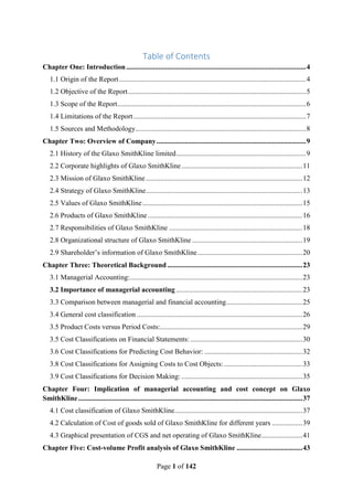
of 142
Chapter Five: Cost-volume Profit analysis of Glaxo
SmithKline
5.1 Fundamental concept of Cost – Volume – Profit Analysis:
Cost-Volume-Profit (CVP) analysis is a managerial accounting technique that is concerned
with the effect of sales volume and product costs on operating profit of a business. It deals with
how operating profit is affected by changes in variable costs, fixed costs, selling price per unit
and the sales mix of two or more different products.
CVP analysis has following assumptions:
 All cost can be categorized as variable or fixed.
 Sales price per unit, variable cost per unit and total fixed cost are constant.
 All units produced are sold.
Cost-volume-profit (CVP) analysis is a powerful tool that helps managers understand the
relationships among cost, volume, and profit. CVP analysis focuses on how profits are affected
by the following five factors:
Figure 14: Five factors of CVP analysis
•Saling
Price
•Sales
Volume
•Unit
Variable
Cost
•Total
Fixed
Cost
•Mix of
Products
Sold

of 142
5.1.1 Overview of Cost-Volume Profit Analysis:
To formally start the discussion of CVP analysis, we will take the help of a contribution format
income statement giving below:
Figure 15: Contribution format income statement
Notice that sales, variable expenses, and contribution margin are expressed on a per unit basis
as well as in total on this contribution income statement. Per unit figures will be very helpful
to SMGK Corporation in some of his calculations. Note that this contribution income statement
has been prepared for management’s use inside the company and would not ordinarily be made
available to those outside the company.
Contribution Margin:
As explained in the previous chapter, contribution margin is the amount remaining from sales
revenue after variable expenses have been deducted. Thus, it is the amount available to cover
fixed expenses and then to provide profits for the period. Notice the sequence here—
contribution margin is used first to cover the fixed expenses, and then whatever remains goes
toward profits. If the contribution margin is not sufficient to cover the fixed expenses, then a
loss occurs for the period. To illustrate with an extreme example, assume that SMGK
Corporation. Sells only one speaker during a particular month. The company’s income
statement would appear as follows:
SMGK Corporation

of 142
Figure 16: Contribution Income Statement
For each additional speaker the company sells during the month, $100 more in contribution
margin becomes available to help cover the fixed expenses. If a second speaker is sold, for
example, then the total contribution margin will increase by $100 (to a total of $200) and the
company’s loss will decrease by $100, to $34,800:
If enough speakers can be sold to generate $35,000 in contribution margin, then all of the fixed
expenses will be covered and the company will break even for the month—that is, it will show
neither profit nor loss but just cover all of its costs. To reach the breakeven point, the company
will have to sell 350 speakers in a month because each speaker sold yields $100 in contribution
margin:
Computation of the break-even point is discussed in detail later in the chapter; for the moment,
note that the break-even point is the level of sales at which profit is zero. Once the break-even

of 142
point has been reached, net operating income will increase by the amount of the unit
contribution margin for each additional unit sold. For example, if 351 speakers are sold in a
month, then the net operating income for the month will be $100 because the company will
have sold 1 speaker more than the number needed to break even:
If 352 speakers are sold (2 speakers above the break-even point), the net operating income for
the month will be $200. If 353 speakers are sold (3 speakers above the breakeven point), the
net operating income for the month will be $300, and so forth. To estimate the profit at any
sales volume above the break-even point, simply multiply the number of units sold in excess
of the break-even point by the unit contribution margin.
The result represents the anticipated profits for the period. Or, to estimate the effect of a planned
increase in sales on profits, simply multiply the increase in units sold by the unit contribution
margin. The result will be the expected increase in profits. To illustrate, if SMGK Corporation.
is currently selling 400 speakers per month and plans to increase sales to 425 speakers per
month, the anticipated impact on profits can be computed as follows:

of 142
These calculations can be verified as follows:
To summarize, if sales are zero, the company’s loss would equal its fixed expenses. Each unit
that is sold reduces the loss by the amount of the unit contribution margin. Once the break-even
point has been reached, each additional unit sold increases the company’s profit by the amount
of the unit contribution margin.
5.1.2 CVP Relationships in Equation Form:
For example, on page 121 we computed the net operating income (profit) at sales of 351
speakers as $100. We can arrive at the same conclusion using the above equation as follows:

of 142
We could also have used this equation to determine the profit at sales of 351 speakers as
follows:
For those who are comfortable with algebra, the quickest and easiest approach to solving the
problems in this chapter may be to use the simple profit equation in one of its forms.
5.1.3 CVP Relationships in Graphic Form:
The relationships among revenue, cost, profit, and volume are illustrated on a cost volume
profit (CVP) graph. A CVP graph highlights CVP relationships over wide ranges of activity.
To help explain his analysis to Pantho Sarker prepared a CVP graph for Acoustic Concepts.
Preparing the CVP Graph:
In a CVP graph (sometimes called a break-even chart), unit volume is represented on the
horizontal (X) axis and dollars on the vertical (Y) axis. Preparing a CVP graph involves three
steps as depicted in Exhibit 4–1:
1. Draw a line parallel to the volume axis to represent total fixed expense. For SMGK
Corporation., total fixed expenses are $35,000.
2. Choose some volume of unit sales and plot the point representing total expense (fixed and
variable) at the sales volume you have selected. In Exhibit 4–1, SMGK Corporation chose a
volume of 600 speakers. Total expense at that sales volume is:

of 142
Figure 17: Preparing CVP graph
Figure 18: The completed graph
After the point has been plotted, draw a line through it back to the point where the fixed expense
line intersects the dollars axis.
3. Again choose some sales volume and plot the point representing total sales dollars at the
activity level you have selected. In Exhibit 4–1, SMGK Corporation again chose a volume of
600 speakers. Sales at that sales volume total $150,000 (600 speakers @ $250 per speaker).

of 142
Draw a line through this point back to the origin. The interpretation of the completed CVP
graph is given in Exhibit 4–2. The anticipated profit or loss at any given level of sales is
measured by the vertical distance between the total revenue line (sales) and the total expense
line (variable expense plus fixed expense). The break-even point is where the total revenue and
total expense lines cross. The break-even point of 350 speakers in Exhibit 4–2 agrees with the
break-even point computed earlier. As discussed earlier, when sales are below the break-even
point—in this case, 350 units— the company suffers a loss. Note that the loss (represented by
the vertical distance between the total expense and total revenue lines) gets bigger as sales
decline. When sales are above the break-even point, the company earns a profit and the size of
the profit (represented by the vertical distance between the total revenue and total expense
lines) increases as sales increase. An even simpler form of the CVP graph, which we call a
profit graph, is presented in Exhibit 4–3. That graph is based on the following equation:
Profit = Unit CM ×Q -Fixed expenses
In the case of Acoustic Concepts, the equation can be expressed as:
Profit = $100×Q -$35,000
Because this is a linear equation, it plots as a single straight line. To plot the line, compute the
profit at two different sales volumes, plot the points, and then connect them with a straight line.
For example, when the sales volume is zero (i.e., Q =0), the profit is -$35,000 (=$100×0-
$35,000). When Q is 600, the profit is $25,000 (=$100× 600-$35,000). These two points are
plotted in Exhibit 4–3 and a straight line has been drawn through them. The break-even point
on the profit graph is the volume of sales at which profit is zero and is indicated by the dashed
line on the graph. Note that the profit steadily increases to the right of the break-even point as
the sales volume increases and that the loss becomes steadily worse to the left of the break-
even point as the sales volume decreases.
5.1.4 Contribution Margin Ratio (CM Ratio):
In the previous section, we explored how cost-volume-profit relationships can be visualized.
In this section, we show how the contribution margin ratio can be used in cost- volume-profit
calculations. As the first step, we have added a column to Acoustic Concepts’ contribution
format income statement in which sales revenues, variable expenses, and contribution margin
are expressed as a percentage of sales:

of 142
The contribution margin as a percentage of sales is referred to as the contribution margin ratio
(CM ratio). This ratio is computed as follows:
Target Profit Analysis:
One of the key uses of CVP analysis is called target profit analysis. In target profit analysis,
we estimate what sales volume is needed to achieve a specific target profit. For example,
suppose that Sajid Hasan of SMGK Corporation would like to know what sales would have to
be to attain a target profit of $40,000 per month. To answer this question, we can proceed using
the equation method or the formula method.
The equation method:
We can use a basic profit equation to find the sales volume required to attain a target profit. In
the case of Acoustic Concepts, the company has only one product so we can use the
contribution margin form of the equation. Remembering that the target profit is $40,000, the
unit contribution margin is $100, and the fixed expense is $35,000, we can solve as follows:
Thus, the target profit can be achieved by selling 750 speakers per month.
The Formula Method:
The formula method is a short-cut version of the equation method. Note that in the next to the
last line of the above solution, the sum of the target profit of $40,000 and the fixed expense of
$35,000 is divided by the unit contribution margin of $100. In general, in a single-product

of 142
situation, we can compute the sales volume required to attain a specific target profit using the
following formula:
Break-Even Analysis:
Earlier in the chapter we defined the break-even point as the level of sales at which the
company’s profit is zero. What we call break-even analysis is really just a special case of target
profit analysis in which the target profit is zero. We can use either the equation method or the
formula method to solve for the break-even point, but for brevity we will illustrate just the
formula method. The equation method works exactly like it did in target profit analysis. The
only difference is that the target profit is zero in break-even analysis.
Break-Even in Unit Sales:
In a single product situation, recall that the formula for the unit sales to attain a specific target
profit is:

of 142
Thus, as we determined earlier in the chapter, Acoustic Concepts breaks even at sales of 350
speakers per month.
Break-Even in Sales Dollars:
We can find the break-even point in sales dollars using several methods. First, we could solve
for the break-even point in unit sales using the equation method or the formula method and
then multiply the result by the selling price. In the case of Acoustic Concepts, the break-even
point in sales dollars using this approach would be computed as 350 speakers× $250 per
speaker or $87,500 in total sales. We can also solve for the break-even point in sales dollars at
Acoustic Concepts using the basic profit equation stated in terms of the contribution margin
ratio or we can use the formula for the target profit. Again, for brevity, we will use the formula.
Operating Leverage:
A lever is a tool for multiplying force. Using a lever, a massive object can be moved with only
a modest amount of force. In business, operating leverage serves a similar purpose.
Operating leverage is a measure of how sensitive net operating income is to a given percentage
change in dollar sales. Operating leverage acts as a multiplier. If operating leverage is high, a

of 142
small percentage increase in sales can produce a much larger percentage increase in net
operating income. Operating leverage can be illustrated by returning to the data for the two
blueberry farms. We previously showed that a 10% increase in sales (from $100,000 to
$110,000 in each farm) results in a 70% increase in the net operating income of Sterling Farm
(from $10,000 to $17,000) and only a 40% increase in the net operating income of Bogside
Farm (from $10,000 to $14,000). Thus, for a 10% increase in sales, Sterling Farm experiences
a much greater percentage increase in profits than does Bogside Farm. Therefore, Sterling Farm
has greater operating leverage than Bogside Farm.
The degree of operating leverage at a given level of sales is computed by the following formula:
Degree of operating leverage =(Contribution Margin)/(Net operating Income)
The degree of operating leverage is a measure, at a given level of sales, of how a percentage
change in sales volume will affect profits. To illustrate, the degree of operating leverage for the
two farms at $100,000 sales would be computed as follows:
Bogside Farm: $40,000/$10,000 = 4
Sterling Farm: $70,000/($10,000 ) = 7
Because the degree of operating leverage for Bogside Farm is 4, the farm’s net operating
income grows four times as fast as its sales. In contrast, Sterling Farm’s net operating income
grows seven times as fast as its sales. Thus, if sales increase by 10%, then we can expect the
net operating income of Bogside Farm to increase by four times this amount, or by 40%, and
the net operating income of Sterling Farm to increase by seven times this amount, or by 70%.
Basically these are the very commonly used tools of CVP analysis. So, these core things have
been discussed in this part of theoretical analysis. The application of all the tools of CVP
analysis are shown in the next part on the five year data set of Glaxo SmithKline.

of 142
5.2 Implication of CVP analysis on Glaxo SmithKline
The part of this chapter will lead the readers to get fullest information regarding the Cost-
Volume Profit Relationship analysis in the aspect of Glaxo SmithKline.
The following table is calculated on the basis of company database to find out the CM ratio
and other tools that will be covered later and step by step:
We can calculate contribution margin and contribution margin ratio of Glaxo SmithKline using
following formula:
Contribution margin: Sales- Variable cost
Contribution ratio=
𝑪𝒐𝒏𝒕𝒓𝒊𝒃𝒖𝒕𝒊𝒐𝒏 𝑴𝒂𝒓𝒈𝒊𝒏
𝑺𝒂𝒍𝒆𝒔
Year Number of Units
Sale
CM Ratio Variable expense Ratio
2010 7751 31% 69%
2011 10203 26% 74%
2012 11177 25% 75%
2013 13127 29% 71%
2014 13326 33% 67%

of 142
Here contribution margin ratio of Glaxo SmithKline company for the years of 2010, 2011,
2012, 2013, 2014 are respectively 31%, 26%, 25%, 29%, and 33%. These contribution margin
ratio show the how contribution margin will be affected by change in a total sales for particular
year.
Calculation Break-Even point in Units of Glaxo SmithKline for year 2010 to 2014:
We can calculate Break-even point in units of Glaxo Smith by using following formula:
Break-even point in units =
𝑭𝒊𝒙𝒆𝒅 𝑪𝒐𝒔𝒕
𝑼𝒏𝒊𝒕 𝑪𝒐𝒏𝒕𝒓𝒊𝒃𝒖𝒕𝒊𝒐𝒏 𝑴𝒂𝒓𝒈𝒊𝒏
Year Fixed Cost
(Million TK)
Unit CM Break-Even point in Units
2010 597964 146.706 4076
2011 822281 121.455 6770
2012 1057136 126.267 8372
2013 1387740 151.775 9143
2014 1309687 178.014 7357
1133561
1239207
1,411,283
1,992,344
2,372,217
0
500000
1000000
1500000
2000000
2500000
2010 2011 2012 2013 2014
Contribution Margin

of 142
Here, break-even point in units of Glaxo SmithKline for year 2010 to 2014 are respectively
4076 units, 6770 units, 8372 units, 9143 units and 7357 units. These respective units must be
sold by Glaxo SmithKline for the particular period to recover its particular year’s fixed cost.
Calculation Break-Even point in TK of Glaxo SmithKline for year 2010 to 2014:
We can calculate the break-even point in taka of Glaxo SmithKline for the year 2010 to 2014
by using following formula:
Break-even point in Taka =
𝑭𝒊𝒙𝒆𝒅 𝑪𝒐𝒔𝒕
𝑪𝒐𝒏𝒕𝒓𝒊𝒃𝒖𝒕𝒊𝒐𝒏 𝑴𝒂𝒓𝒈𝒊𝒏 𝑹𝒂𝒕𝒊𝒐
Year Fixed Cost
(Million TK)
CM Ratio Break-Even point in TK
(million)
2010 597964 31% 1928916
2011 822281 26% 3162619
2012 1057136 25% 4228544
2013 1387740 29% 4785310
2014 1309687 33% 3968748
4076
6770
8372
9143
7357
0
1000
2000
3000
4000
5000
6000
7000
8000
9000
10000
2010 2011 2012 2013 2014
Break-Even point in Units

of 142
Here, break-even point in taka of Glaxo SmithKline Company for year 2010 to 2014 are
respectively TK. 1928916 million, TK. 3162619 million, TK. 4228544 million, TK. 4785310
million, and TK. 3968748 million. These respective amounts of sales must be sold by Glaxo
SmithKline for the particular period to recover its particular year’s fixed cost.
Calculation of targets units to attain target profits of Glaxo SmithKline for year 2010 t0
2014:
We can calculate the target unit to attain target profits of Glaxo SmithKline by using following
formula:
Break-even point in units =
𝑭𝒊𝒙𝒆𝒅 𝑪𝒐𝒔𝒕 +𝑻𝒂𝒓𝒈𝒆𝒕 𝒑𝒓𝒐𝒇𝒊𝒕
𝑼𝒏𝒊𝒕 𝑪𝒐𝒏𝒕𝒓𝒊𝒃𝒖𝒕𝒊𝒐𝒏 𝑴𝒂𝒓𝒈𝒊𝒏
Year Fixed Cost
(Million)
Target Profit Unit CM Target Units
2010 597964 535597 146.706 7727
2011 822281 416926 121.455 10203
2012 1057136 354147 126.267 11177
1928916
3162619
4228544
4785310
3968748
0
1000000
2000000
3000000
4000000
5000000
6000000
Break-Even point in TK (Million)
2010 2011 2012 2013 2014

of 142
2013 1387740 604604 151.775 13127
2014 1309687 1062350 178.014 13325
Here target units of Glaxo SmithKline Company to attain its expected profit for year 2010 to
2014 are respectively 7727units, 10203 units, 11177 units, 13127 units, and 13325 units. These
respectively units must be sold by Glaxo SmithKline to attain its particular year’s expected
profit.
Calculation of target amounts in Taka to attain target profits of Glaxo SmithKline for
year 2010 to 2014:
We can calculate the target amount in Taka of Glaxo SmithKline to attain its expected profit
Target amounts in Taka =
𝑭𝒊𝒙𝒆𝒅 𝑪𝒐𝒔𝒕 +𝑻𝒂𝒓𝒈𝒆𝒕 𝒑𝒓𝒐𝒇𝒊𝒕
𝑪𝑴 𝒓𝒂𝒕𝒊𝒐
Year Fixed Cost
(Million)
Target Profit
(Million)
CM Ratio Target amounts
in Taka (Million)
2010 597964 535597 31% 3656648
2011 822281 416926 26% 4766181
2012 1057136 354147 25% 5645132
2013 1387740 604604 29% 6870152
2014 1309687 1062350 33% 7187991
Here, target amounts in Taka of Glaxo SmithKline for year 2010 to 2014 are respectively TK.
3656648 million, TK. 4766181 million, TK. 5645132 million, TK. 6870152 million, and TK.
7187991 million. These respective amounts of sales must be sold by Glaxo SmithKline for the
particular period to its expected profit particular year’s fixed cost.

of 142
Calculation of the margin of safety in Taka and percentage form of Glaxo SmithKline for
year 2010 to 2014:
We can calculate the Margin of Safety and Margin of safety percentage of Glaxo SmithKline
Margin of safety = Actual sales – Break-even sales
Margin of safety percentage =
𝑴𝒂𝒓𝒈𝒊𝒏 𝒐𝒇 𝑺𝒂𝒇𝒆𝒕𝒚
𝑨𝒄𝒕𝒖𝒂𝒍 𝒔𝒂𝒍𝒆𝒔
Year Actual
Sales
(Million TK)
Break-Even Sales
(Million TK)
Margin of safety
(Million TK)
Margin of
safety
percentage
2010 3632095 1928916 1703179 46.89%
2011 4735121 3162619 1572502 33.21%
2012 5,553,812 4228544 1325268 23.86%
2013 6,774,872 4785310 1989562 29.37%
2014 7,187,225 3968748 3218477 44.78%
Here margin of safety of Glaxo SmithKline for years 2010 to 2014 are respectively TK.
1703179 million, TK. 1572502 million, TK 1325268 million, TK. 1989562 million, and TK.
3218477 million. These amounts represents, lower risk of not break-even of Glaxo SmithKline
1703179
1572502
1325268
1989562
3218477
0
500000
1000000
1500000
2000000
2500000
3000000
3500000
2010 2011 2012 2013 2014
Margin of safety

of 142
Company. The margin of safety percentage of Glaxo SmithKline for year 2010 to 2014 are
respectively 46.89%, 33.21%, 23.86%, and 44.78%.
Calculation of the Degree of the operating leverage of Glaxo SmithKline for year 2010 to
2014:
We can calculate Degree of the operating leverage of Glaxo SmithKline by using following
formula:
Degree of operating leverage =
𝐶𝑜𝑛𝑡𝑟𝑖𝑏𝑢𝑡𝑖𝑜𝑛 𝑀𝑎𝑟𝑔𝑖𝑛
𝑁𝑒𝑡 𝑜𝑝𝑒𝑟𝑎𝑡𝑖𝑛𝑔 𝐼𝑛𝑐𝑜𝑚𝑒
Year Contribution
Margin
Net operating
Income
Degree of Operating leverage
2010 1133561 535597 2.116443893
2011 1239207 416926 2.972246874
2012 1,411,283 354147 3.985020345
2013 1,992,344 604604 3.295287494
2014 2,372,217 1062350 2.232990069
Here degree of operating leverage of Glaxo SmithKline for year 2010 to 2014 are respectively
2.116443893, 2.972246874, 3.985020345, 3.295287494, and 2.232990069. These degree of
operating leverage measures how a percentages changes in sales volume will affect profits.
Estimation of next year expected net operating income (2015):
We can calculate future expected increase in net operating income by using degree of operating
leverage. For this, we assume future expected increase in sales of Glaxo SmithKline is TK.
412353 million.
Expected increase in sales Degree of operating leverage Expected increase in NOI
412353 2.116443893 872722

of 142
Chapter Six: Variable Costing Analysis
6.1 Fundamental concept of variable costing
Cost Accounting:
Cost accounting is a process of collecting, recording, classifying, analyzing, summarizing,
allocating and evaluating various alternative courses of action & control the cost. Its goal is to
advise the management on the most appropriate course of action based on the cost efficiency
and capability. In other words, costing is any system for assigning costs to an element of a
business. Costing is typically used to develop costs for any or all of the following:
 Customers
 Distribution channels
 Employees
 Geographical regions
 Products
 Product lines
 Processes
 Subsidiaries
 Entire companies
Methods of Costing:
Generally two methods are being used widely in manufacturing companies for costing products
for the purposes of valuing inventories and cost of goods sold. They are:
Figure 19: Methods of costing
Methods
of Costing
Absorption
costing
Variable
costing

of 142
1) Absorption costing
2) Variable costing
Absorption Costing:
Absorption costing treats all manufacturing costs as product costs, regardless of whether they
are variable or fixed. The cost of a unit of product under the absorption costing method consists
of direct materials, direct labor, and both variable and fixed manufacturing overhead. It
includes the assignment of fixed costs, which are those costs that stay the same, irrespective of
the level of activity. This type of costing is also called full cost method costing. Examples of
fixed costs are rent, insurance, and property taxes etc.
Variable Costing:
Under variable costing, only those manufacturing costs that vary with output are treated as
product costs. This would usually include direct materials, direct labor, and the variable portion
of manufacturing overhead. Fixed manufacturing overhead is not treated as a product cost
under this method. Rather, fixed manufacturing overhead is treated as a period cost and, like
selling and administrative expenses. These are the costs that vary with some form of activity
(such as sales or the number of employees). This type of costing is also called direct costing or
marginal costing. For example, the cost of materials varies with the number of units produced,
and so is a variable cost.
Figure 20 Absorption costing Vs. Variable costing

of 142
6.2 Implication of variable costing concept on Glaxo SmithKline
Here, in this part we will use both methods Absorption costing and variable costing for
determining the annual costing amount of Glaxo SmithKline. Required data and information
for implication of variable costing concept are presented below:
Particular Year
2010 2011 2012 2013 2014
Sales price 469 464.09 496.90 516.10 539.34
Direct materials 213 252 259 262 247
Direct labor 18 14 14 15 13
Variable Manufacturing overhead 46.9 46.4 49.6 51.6 53.9
Fixed Manufacturing overhead 15.90 13.40 14.48 15.65 15.20
Variable selling and administrative
expenses
23.45 23.2 24.8 25.8 26.95
Fixed selling and administrative expenses 57.93 62.62 79.47 84.35 72.54
Here, we are assumed variable manufacturing overhead 10% of selling price. We are also
assumed that variable selling and administrative expenses is 5% selling price.
Items 2010 2011 2012 2013 2014
Beginning inventory 245913 264809 53508101 52001984 61108481
Production 582293 825906 109352062 108821042 98288811
Sales 3632095 4735121 5,553,812 6,774,872 7,187,225
Ending inventory 419001 264809 52636798 53508101 52001984
We will first construct the company’s absorption costing income statements for 2010, 2011,
2012, 2013 and 2014. Then we will show how the company’s net operating income would be
determined for the same months using variable costing.

of 142
Absorption costing unit product cost
Items 2010 2011 2012 2013 2014
Variable manufacturing overhead 46.9 46.4 49.6 51.6 53.9
Fixed manufacturing overhead 15.90 13.40 14.48 15.65 15.20
Absorption costing unit product cost 293.80 325.80 337.08 344.25 329.10
Given these unit product costs, the cost of goods sold under absorption costing in each year
would be determined as follows:
Items 2010 2011 2012 2013 2014
Absorption costing unit
product cost
293.80 325.80 337.08 344.25 329.10
Units sold 7751 10203 11177 13127 13326
Absorption costing cost
of goods sold
227724.80 3324137.40 3767543.16 4518970 4385586.6
Selling and Administrative Expenses
Items 2010 2011 2012 2013 2014
Variable selling and
administrative expense
181760.95 236709.60 277189.60 338676.6 359135.70
Fixed selling and
449015.43 638911.86 888236.19 1107262.45 966668.04
Total selling and
630776.38 875621.46 1165425.79 1445939.05 1325803.74
Putting all of this together, the absorption costing income statements would appear as:
Items 2010 2011 2012 2013 2014
Sales 3632095 4735121 5,553,812 6,774,872 7,187,225
Cost of goods sold (227724.80) (3324137.40) (3767543.16) (4518970) (4385586.6)
Gross margin 3404370.20 1410984 1786268.84 2255902 2801638.40
Selling and
administrative
expenses
630776.38 875621.46 1165425.79 1445939.05 1325803.74
Net operating
income (loss)
2773594 535362.54 620843.05 809962.95 1475834.66

of 142
Variable Costing Contribution Format Income Statement:
In variable costing, fixed manufacturing overhead is not included in product costs and instead
is treated as a period expense, just like selling and administrative expenses:
Variable costing unit product cost
Items 2010 2011 2012 2013 2014
Variable manufacturing
overhead
46.9 46.4 49.6 51.6 53.9
Variable costing unit
product cost
277.90 312.4 322.60 328.6 313.90
The variable costing cost of goods sold can be easily computed using this unit product cost as
follows:
Variable Cost of goods sold
Items 2010 2011 2012 2013 2014
Variable costing
unit product cost
277.90 312.4 322.60 328.6 313.90
Units sold 7751 10203 11177 13127 13326
Variable cost of
goods sold
2154002.90 3187417.20 3605700.2 4313532.2 4183031.4
The selling and administrative expenses will be the same as the amounts reported using
absorption costing. The only difference will be how those costs appear on the income statement
The variable costing income statements for year 2010 to 2014 appear in the following chart.
The contribution format has been used in these income statements.

of 142
Variable costing Income statement
Items 2015 2014 2013 2012 2011
Sales 3632095 4735121 5,553,812 6,774,872 7,187,225
Variable cost of
goods sold
(2154002.90) (3187417.20) (3605700.2) (4313532.2) (4183031.4)
Variable selling and
administrative
expense
(181760.95) (236709.60) (277189.60) (338676.6) (359135.70)
Contribution
margin
1296331.15 1310994.2 1670922.20 2122663.2 2645057.90
Fixed
manufacturing
overhead
(123240.9) (136720.20) (161842.96) (205437.55) (206553)
Fixed selling and
administrative
expense
(449015.43) (638911.86) (888236.19) (1107262.45) (966668.04)
Net operating
income (loss)
724074.82 535362.14 620843.05 809963,20 1471836.86
The format of the variable costing income statement differs from the absorption costing income
statement. An absorption costing income statement categorizes costs by function—
manufacturing versus selling and administrative. All of the manufacturing costs flow through
the absorption costing cost of goods sold and all of the selling and administrative costs are
listed separately as period expenses. In contrast, in the contribution approach above, costs are
categorized according to how they behave. All of the variable expenses are listed together and
all of the fixed expenses are listed together.

of 142
6.3 Comparative Income Effects—Absorption and Variable Costing
Variable costing and absorption costing usually produce different net operating income figures.
The reason is that the fixed manufacturing overhead cost is not treated the same way under two
costing methods. The key points in these topics are:
 The net operating income under absorption costing systems is always higher than
variable costing system when inventory increases.
 The net operating income under variable costing systems is always higher
than absorption costing system when inventory decreases.
 When inventory increases, the fixed manufacturing overhead cost is deferred to
inventory.
 When inventory decreases, the fixed manufacturing overhead cost is released from
inventory.
In the following a chart on comparative income effects of Absorption and variable costing is
given below:
Situations Variable costing Absorption costing Effect on inventories
Production = Sales Equal Equal Equal
Production > Sales Lower Higher Increase
Production < Sales Higher Lower Decrease
In this chart,
 When production exceeds sales net operating income is higher under absorption costing
because fixed manufacturing overhead cost is ‘deferred’ in inventory under absorption
costing as inventories increase.
 When sales exceeds production Net operating income is lower under absorption costing
because fixed manufacturing overhead cost is ‘released’ from inventory under
absorption costing as inventories decrease.

of 142
6.4 Comparative Advantages of Variable costing:
Even if the absorption approach is used for external reporting purposes, variable costing,
together with the contribution format income statement, is an appealing alternative for internal
reports. The advantages of variable costing can be summarized as follows:
 Data required for CVP analysis can be taken directly from a contribution format income
statement. These data are not available on a conventional absorption costing income
statement.
 Under variable costing, the profit for a period is not affected by changes in inventories.
Other things remaining the same (selling prices, costs, sales mix, etc.), profits move in
the same direction as sales when variable costing is used.
 Managers often assume that unit product costs are variable costs. This is a problem
under absorption costing because unit product costs are a combination of both fixed and
variable costs. Under variable costing, unit product costs do not contain fixed costs.
 The impact of fixed costs on profits is emphasized under the variable costing and
contribution approach. The total amount of fixed costs appears explicitly on the income
statement, highlighting that the whole amount of fixed costs must be covered for the
company to be truly profitable. In contrast, under absorption costing, the fixed costs are
mingled together with the variable costs and are buried in cost of goods sold and ending
inventories.
 Variable costing data make it easier to estimate the profitability of products, customers,
and other business segments. With absorption costing, profitability is obscured by
arbitrary fixed cost allocations. These issues will be discussed in later chapters.
 Variable costing ties in with cost control methods such as standard costs and flexible
budgets, which will be covered in later chapters.
 Variable costing net operating income is closer to net cash flow than absorption costing
net operating income. This is particularly important for companies with potential cash
flow problems.

of 142
Chapter Seven: Activity based Costing Analysis
7.1 Fundamental concept of activity based costing
Activity Based Costing: An overview:
Activity-based costing (ABC) is a costing methodology that identifies activities in an
organization and assigns the cost of each activity with resources to all products and services
according to the actual consumption by each. This model assigns more indirect costs (overhead)
into direct costs compared to conventional costing.
Activity based costing (ABC) assigns manufacturing overhead costs to products in a more
logical manner than the traditional approach of simply allocating costs on the basis of machine
hours. Activity based costing first assigns costs to the activities that are the real cause of the
overhead. It then assigns the cost of those activities only to the products that are actually
demanding the activities.
Activity based costing has grown in importance in recent decades because (1) manufacturing
overhead costs have increased significantly, (2) the manufacturing overhead costs no longer
correlate with the productive machine hours or direct labor hours, (3) the diversity of products
and the diversity in customers' demands have grown, and (4) some products are produced in
large batches, while others are produced in small batches.
According to CIMA (Chartered Institute of Management Accountants):
ABC is acted as an approach to the costing and monitoring of activities which involves tracing
resource consumption and costing final outputs. Resources are assigned to activities, and
activities to cost objects based on consumption estimates. The latter utilize cost drivers to attach
activity costs to outputs.

of 142
Objectives:
With ABC, a company can soundly estimate the cost elements of entire products, activities and services.
That may help inform a company's decision to either:
Identify and eliminate those products and services that are unprofitable and lower the prices of
those that are overpriced (product and service portfolio aim)
Or identify and eliminate production or service processes that are ineffective and allocate
processing concepts that lead to the very same product at a better yield (process re-engineering
aim
In a business organization, the ABC methodology assigns an organization's resource costs through
activities to the products and services provided to its customers. ABC is generally used as a tool for
understanding product and customer cost and profitability based on the production or performing
processes. As such, ABC has predominantly been used to support strategic decisions such as pricing,
outsourcing, identification and measurement of process improvement initiatives.
Methodology:
Methodology of ABC focuses on cost allocation in operational management. ABC helps to
segregate
 Fixed cost
 Variable cost
 Overhead cost
The split of cost helps to identify cost drivers, if achieved. Direct labor and materials are
relatively easy to trace directly to products, but it is more difficult to directly allocate indirect
costs to products. Where products use common resources differently, some sort of weighting
is needed in the cost allocation process. The cost driver is a factor that creates or drives the
cost of the activity. For example, the cost of the activity of bank tellers can be ascribed to each
product by measuring how long each product's transactions (cost driver) takes at the counter
and then by measuring the number of each type of transaction. For the activity of running
machinery, the driver is likely to be machine operating hours. That is, machine operating hours’
drive labor, maintenance, and power cost during the running machinery activity.
Application of the ABC Costing:

of 142
ABC has proven its applicability beyond academic discussion. ABC is applicable throughout
company financing, costing and accounting:
 ABC is a modeling process applicable for full scope as well as for partial views.
 ABC helps to identify inefficient products, departments and activities.
 ABC helps to allocate more resources on profitable products, departments and activities.
 ABC helps to control the costs at any per-product-level level and on a departmental level.
 ABC helps to find unnecessary costs that may be eliminated.
 ABC helps fixing the price of a product or service with any desired analytical resolution.
A report summarizes reasons for implementing ABC as mere unspecific and mainly for case
study purposes.
 Budgeting, performance measurement
 Better Management
 Calculating costs more accurately
 Ensuring product /customer profitability
 Evaluating and justifying investments in new technologies
 Improving product quality via better product and process design
 Increasing competitiveness or coping with more competition
 Management
 Managing costs
 Providing behavioral incentives by creating cost consciousness among employees
 Responding to an increase in overheads
 Responding to increased pressure from regulators
 Supporting other management innovations such as TQM and JIT systems
Beyond such selective application of the concept, ABC may be extended to accounting, hence
proliferating a full scope of cost generation in departments or along product manufacturing.
Such extensions, however requires a degree of automatic data capture that prevents from cost
increase in administering costs.
Cost Hierarchy in Activity-Based Costing:

of 142
Thousands of activities are carried out in most organizations. It would not be practical to track
all of them in an activity-based costing system. A great deal of simplification is necessary.
Activities and their costs must be combined to reduce complexity and record-keeping
requirements. One way to simplify is to group activities into a hierarchy. Activities, and their
costs, can be combined within each level of the hierarchy into activity cost pools—hopefully
with minimal loss in accuracy. The cost hierarchy used in the text is not the only scheme that
could be used, but it is reasonably comprehensive. The levels in the hierarchy are as follows:
Unit-level activities: These activities are performed each time a unit is produced. For example,
providing power to run processing equipment is likely to be a unit-level activity.
Batch-level activities: These activities are performed each time a batch is handled or
processed, regardless of how many units are in the batch. For example, tasks such as placing
purchase orders, setting up equipment, and arranging for shipments to customers are batch-
level activities.
Product-level activities: These activities relate to specific products and must be carried out
regardless of how many batches or units of product are produced or sold. For example,
designing a product, advertising a product, and maintaining a product manager and staff are all
product-level activities.
Customer-level activities: These activities relate to specific customers and include sales calls,
catalog mailings, and general technical support not tied to any specific product.
Organization-sustaining activities: These activities are carried out regardless of which
products are produced, how many batches are run, or how many units are made. This category
of activities includes cleaning executive offices, providing a computer network, arranging for
loans, preparing annual reports to shareholders, and so on.
Designing an Activity Based Costing System:
An action analysis report makes it much clearer what costs are likely to be relevant in a decision
and who in the organization would be responsible for the cost if an action is taken.
Unfortunately, preparing an action analysis report requires considerably more work than the
more conventional analysis.

of 142
1. Activity rates: The action analysis approach differs from the conventional ABC approach
beginning with the computation of the activity rates. In the conventional analysis, a single
activity rate is computed for each activity cost pool. In an action analysis, a rate is computed
for each cost category within an activity cost pool. Looking at Exhibit 8A-2, only the rates at
the bottom of the Exhibit would be computed in a conventional analysis. In an action analysis,
the entire table is filled out.
2. Assign overhead cost to activity cost pools: In an action analysis, an entire matrix of costs
is computed rather than just a total cost for each activity cost pool. Looking at Exhibit 8A-3,
only the costs at the bottom of the Exhibit would be computed in a conventional analysis. In
an action analysis, the entire table is filled out by multiplying activities by the activity rates in
each cell.
3. The conventional activity rate analysis: From the action analysis cost matrix in Exhibit
8A-3, it is easy to construct the conventional activity analysis report showing product margins.
Just take the totals from the bottom of the cost matrix.
However, using the row totals from Exhibit 8A-3, it is possible to look at the margins of
products and other cost objects from a different perspective. Instead of abstract labels like
“order processing costs” for the various activity cost pools, the costs are labeled using the
account titles from the company’s bookkeeping system. This makes it clear what the costs
actually consist of and who in the organization would be responsible for taking action if a
decision is made.
4. Assign overhead cost to cost objects using the activity rate: sand activity measure: Some
costs, such as direct materials, are much easier to adjust than other costs, such as the total wages
of experienced supervisors. As a consequence, some costs are more likely to be relevant in a
decision than others. The ease of adjustment codes provide a way of assisting managers in
making these distinctions.
5. Prepare Management report: The action analysis report combines the cost information
from the row totals in Exhibit 8A-3 with the ease of adjustment codes in Exhibit 8A-4. This
report makes it much clearer where costs would need to be adjusted in the organization as the
result of an action, who would be responsible for the change in costs, and which costs are likely
to be relevant and which costs are likely to be irrelevant in decisions. Such an action analysis

of 142
report is not the final step in the decision-making process. Further analysis, such as illustrated
in Chapter 13, would be necessary before making any major decision.
Advantages of Activity-Based Costing
Improves Business Processes: An ABC system allocates indirect costs based on a product’s
cost driver, or the factor that creates the cost. As costs are allocated per product, a picture starts
to emerge of which business processes are performing well and which ones need to be
improved. ABC can be used to identify non-valued added activities and can help to better
allocate resources to efficient and profitable activities. The use of ABC can also add value to
the continuous improvement of business processes.
Identifies Wasteful Products: The ABC method accounts for costs similar to the way
production work is performed, allowing your business to better understand where overhead
costs are going. The data can identify wasteful products and unnecessary costs, so that
resources can be used productively. The method also helps to fix the price of products or
services that are excessive or incorrect. Overall product and service quality can improve as
ABC’s data details production and cost issues that need to be resolved.
Pricing Is Better Organized: With ABC businesses are able to fully identify all the costs that
are associated with producing a single unit of their product. Because of this new understanding,
they are able to develop pricing strategies and marketing much more efficiently.
Can Be Applied To The Entire Business: It may seem that activity based costing is only
effective and efficient for the production costs that are involved in a business, but all overhead
costs can be reduced using this method. Everything from management, CEO’s, and entry level
employees.

of 142
The limitations of Activity-Based Costing
Activity-based costing is a way to allocate costs based on the amount of resources a product or
service consumes. The use of ABC is especially important to businesses that provide
customized products or services. A customized production environment requires ABC’s
allocation of actual indirect costs to a product to identify its true cost. Implementing ABC can
be a challenging task for any business and the process carries several advantages and
disadvantages.
Expensive Implementation: Setting up an ABC system can be expensive and time-
consuming. As business activities are analyzed, they must be broken down into each activity’s
individual components. The entire process can use up valuable resources as data are collected,
measured and entered into the new system. Businesses may also need the assistance of a
consultant who specializes in the setup of an ABC system and can provide training on its use.
Using software can add an additional expense to the implementation but it can be used to
automate many of the manual aspects involved in using ABC.
Misinterpretation of Data: Reports produced by an ABC system contain information, such
as product margins, that vary from the information reported for a traditional cost method. It’s
also possible that some activity-based costs may be irrelevant in certain decision-making
scenarios; for example, ABC does not conform to accounting standards and should not be used
for external reporting. Since traditional cost figures tend to be the norm, interpreting ABC data
along with regular accounting information can be confusing and lead to bad decision-making.
The use of software can streamline the process of maintaining an ABC system and simplify its
integration with regular cost accounting information.
Reduction Is Not Always Possible: If the overhead costs are high for reasons such as volume,
there are very limited benefits to be reaped from activity based costing. It also is not very
efficient if the overhead costs of the business only represent a very small portion of the costs.
High Implementation Costs: ABC method of costs may not be best if the overhead waste is
perceived to be relatively low. This is because it can be very costly to implement activity based
costing into a business. Experts must be brought in for an extended period of time, and other
measures may be necessary for the ABC to be effective.

of 142
Time Involved: There is a long time period that is involved in using an activity based costing
method in a business. All of the production processes, employee actions, and aspects of the
business have to be examined for an extended period of time in order to gain a big view on
what the issues truly are.
Data Flaws: ABC requires many different departments and individuals to collect and input data.
Even the smallest flaw in this information can damage the entire process and the outcome
would be tainted. This is one of the biggest risks that are taken on when using this method.

of 142
7.2 Implication of activity based costing on Glaxo SmithKline
Assumptions:
1. We assumed factory overhead cost as it was not available in company’s financial
statement directly.
2. The company produce several products. But we take only two products for our analysis.
3. Activity is assumed, as it is not available in the financial statements of the company.
Step-1 assign annual overhead costs:
This is the first stage of the ABC costing. The last five years’ data have been collected and we
tried to find out the annual average cost of 2015, 2014,2013,2012,2011. So this chart shows
the cost of sales, factory overhead, administrative expenses and selling, distribution and
marketing expenses of different years.
Figure 21: Different types of cost
0
1000000
2000000
3000000
4000000
5000000
2014 2013 2012 2011 2010
Different types of cost
cost of sales factory overhead
administrative expenses selling, distribution expenses

of 142
Now here we show mathematically assign annual overhead cost for the different years.
Year 2014:
Annual overhead cost for 2014
TK
cost of sales 4476255
factory overhead 900000
administrative expenses 334467
selling, distribution expenses 1325952
total overhead cost 7036674
Year 2013:
TK

of 142
Year 2012:
Year 2011:
Year 2010:
Annual overhead cost for
2010

of 142
Stage-2: assign overhead costs to activity cost pools same for all the years:
This chart shows the total contribution of cost of sales, factory overhead, administrative
expenses and selling, distribution and market expense of the GlaxoSmithKline Bangladesh
Limited.
One important note is that this chart of activity cost pool remain same all the years so that we
can compare easily among last five years. So we assume that the activity cost pool remain
same.
Activity cost pools is same for all the years
customer
order
product
design
order
size
custome
r
relation
other
s
total
cost of sales 25% 40% 20% 10% 5% 100
%
factory overhead 20% 0% 60% 0% 20% 100
%
administrative expenses 15% 5% 10% 30% 40% 100
%
selling, distribution &
marketing expenses
22% 8% 0% 60% 10% 100
%

of 142
Stage-3: allocation to activity cost pools:
Figure 22: Assigning total cost in various cost pools
Here the chart shows the activity cost pool for the last 5 years. Here we find the total amount
spend in customer order, production design, order size and others part.
Figure 23: Activity cost pools
cost of sales factory overhead
administrative
expenses
selling, distribution
& marketing
expenses
2015 178031685 27989142 20014464 132860435
2014 162651431 26582274 18689414 134101621
2013 132352513 25067195 11534569 114267720
2012 124345440 25157246 10820959 113249734
2011 124702163 27075902 10145441 111980881
0
20000000
40000000
60000000
80000000
100000000
120000000
140000000
160000000
180000000
200000000
AXISTITLE
Assigning total cost in various cost pools
0
500000
1000000
1500000
2000000
2500000
2014 2013 2012 2011 2010
Activity cost pool
customer order product design order size customer relation others

of 142
The amount along with total under each cost pools are shown below:
2014 2013 2012 2011 2010
customer order 1640943 1631959 1401709 1177608 873632.7
product design 1913302 1929886 1680036 1423361 1008397
order size 1468698 1415109 1257170 1113604 882520.1
customer relation 1343537 1351875 1091420 841663.2 621797.3
others 670194.8 647058.8 513733.1 450112.6 364291.9
Figure 24: Activity cost pools
In the following, we show mathematical derivation of the amount of customer order, product
design, order size, customer relationship and others.
customer
order
product
design
order size customer
relation
others total
cost of sales 1119063.75 1790502 895251 447625.5 223812.8 4476255
factory overhead 180000 0 540000 0 180000 900000
administrative
expenses
50170.05 16723.35 33446.7 100340.1 133786.8 334467
selling,
distribution
expenses
291709.44 106076.16 0 795571.2 132595.2 1325952
Total 1640943 1913302 1468698 1343537 670194.8 7036674
Figure 25: Activity cost pools for the year 2014
customer
order
product
design
order size customer
relation
others total
cost of sales 1129176.25 1806682 903341 451670.5 225835.3 4516705
factory overhead 160000 0 480000 0 160000 800000
administrative
expenses
47652.6 15884.2 31768.4 95305.2 127073.6 317684
selling,
distribution
expenses
295129.78 107319.92 0 804899.4 134149.9 1341499
Total 1631958.63 1929886.12 1415109.4 1351875.1 647058.8 6975888
Figure 26: Activity cost pool for the year 2013

F-302 Managerial Accounting

Recommended

Recommended

More Related Content

What's hot

What's hot (20)

Similar to F-302 Managerial Accounting

Similar to F-302 Managerial Accounting (20)

More from Pantho Sarker

More from Pantho Sarker (20)

Recently uploaded

Recently uploaded (20)

F-302 Managerial Accounting