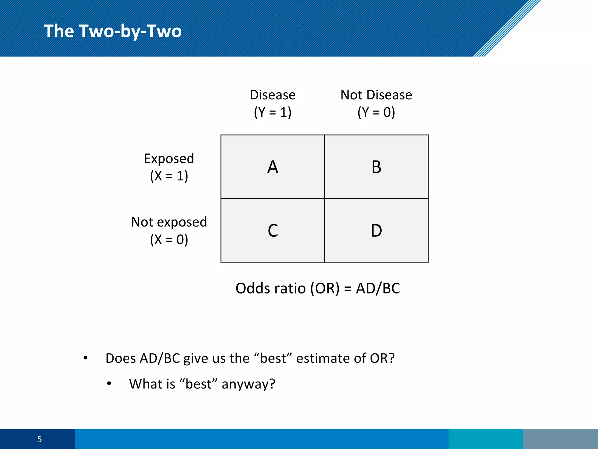
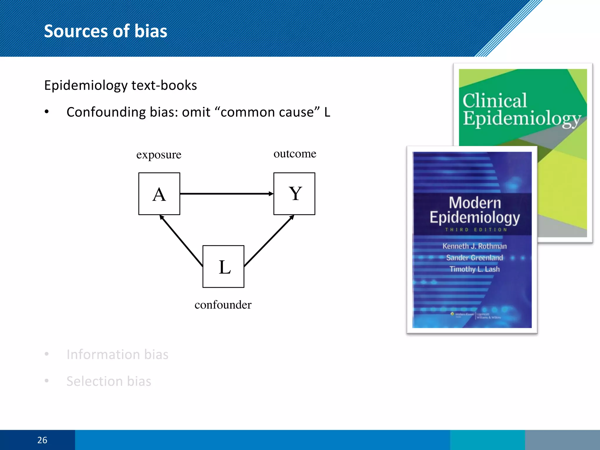
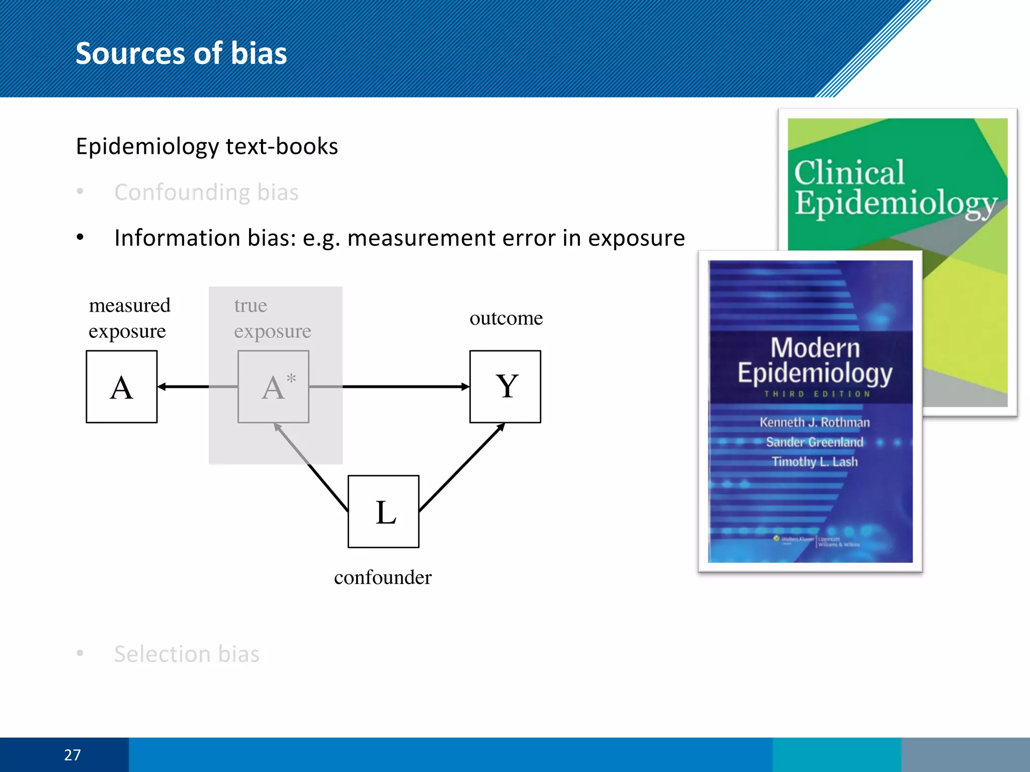
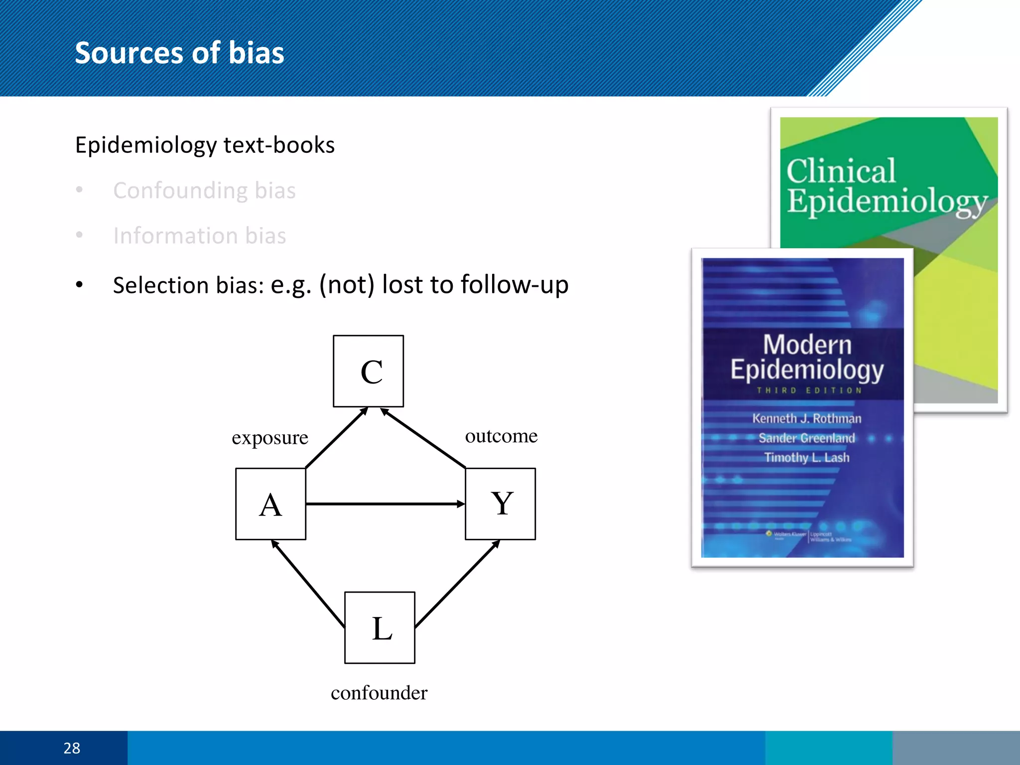
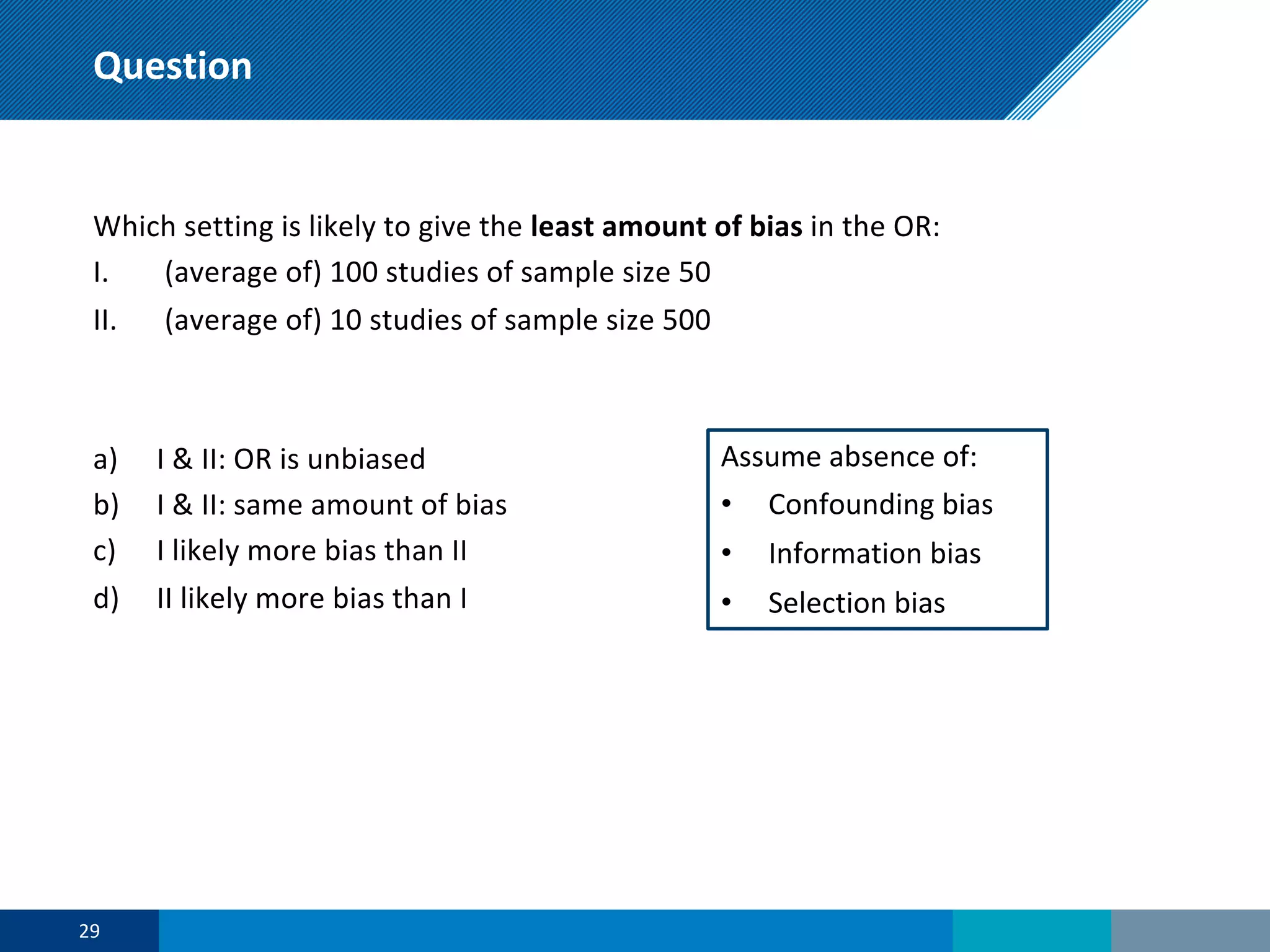
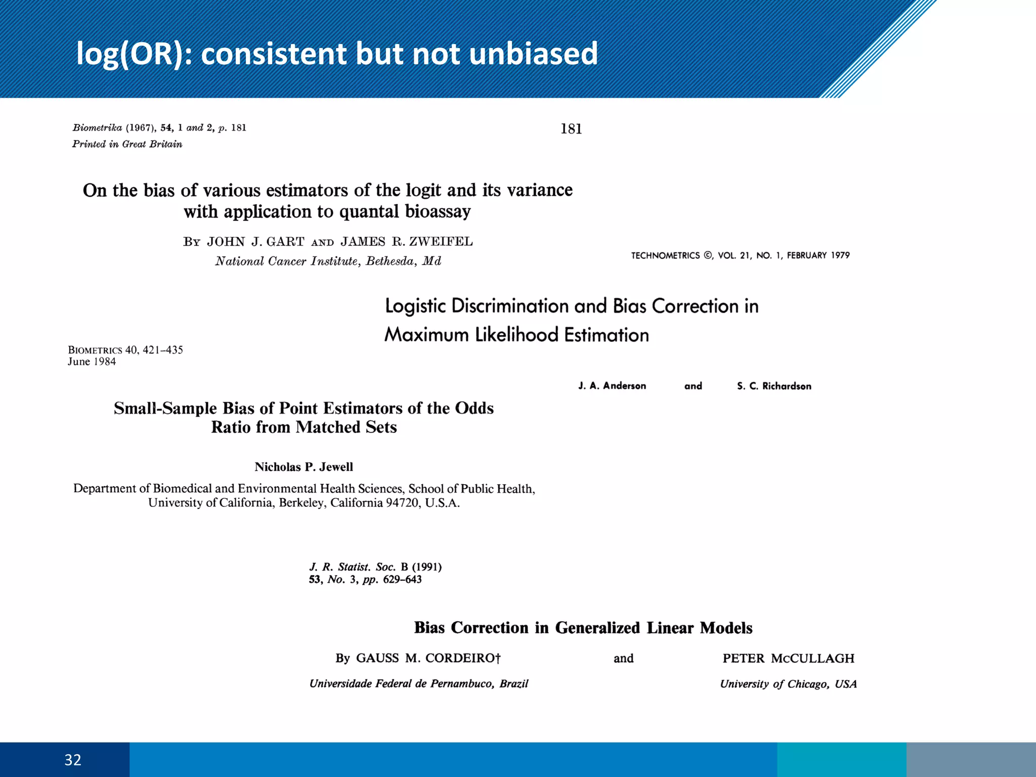
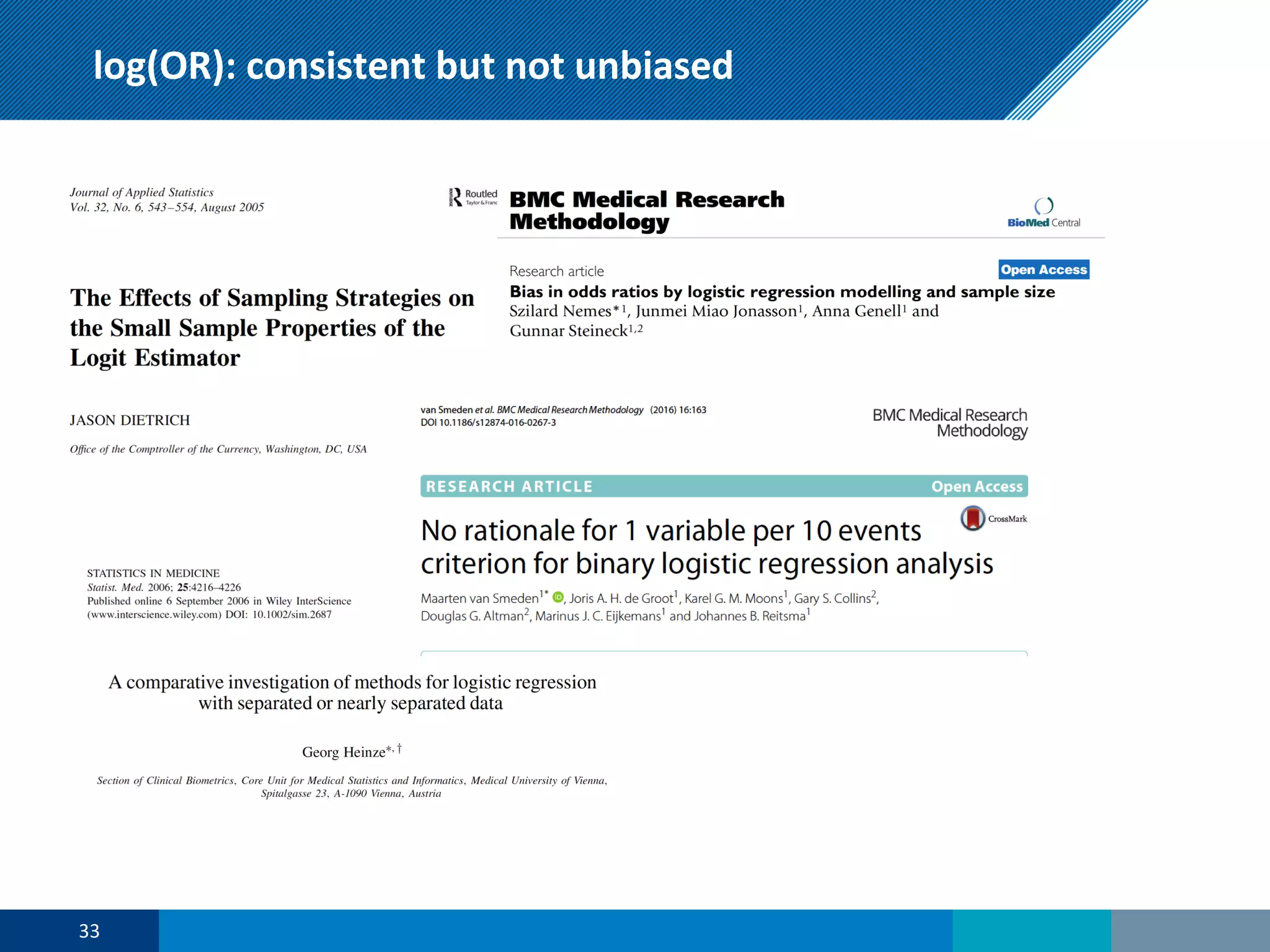
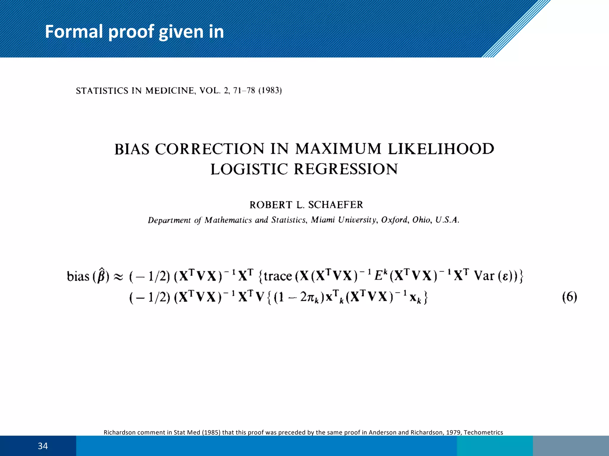
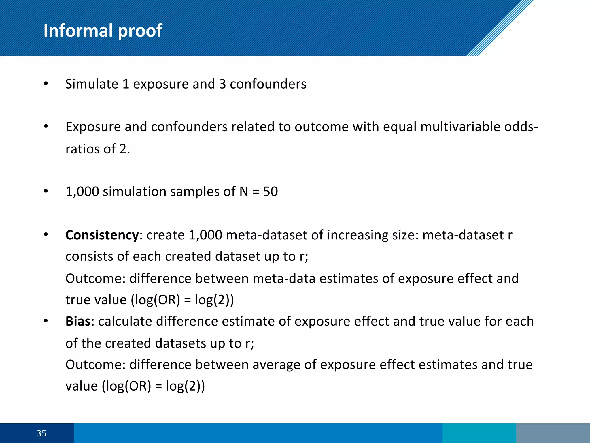
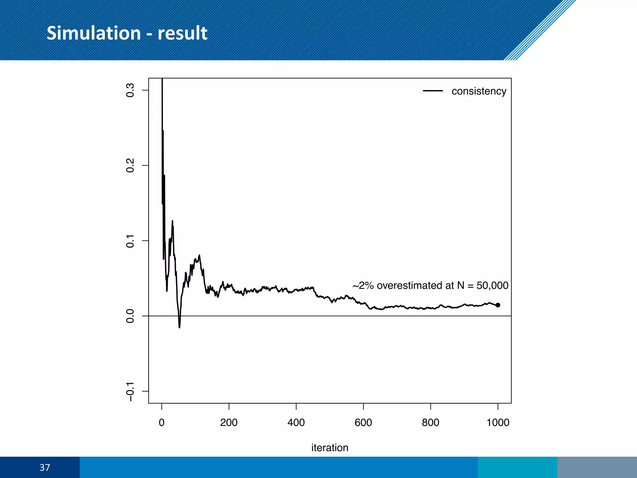
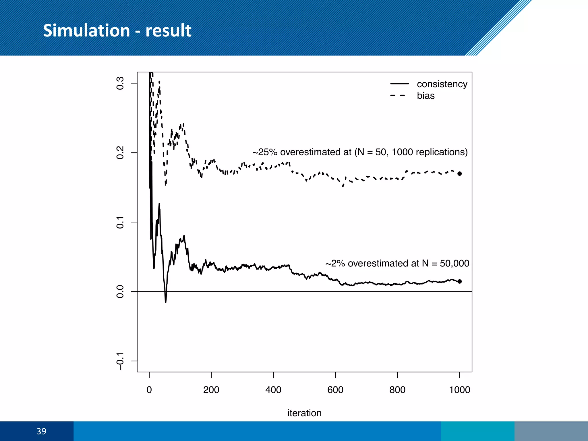
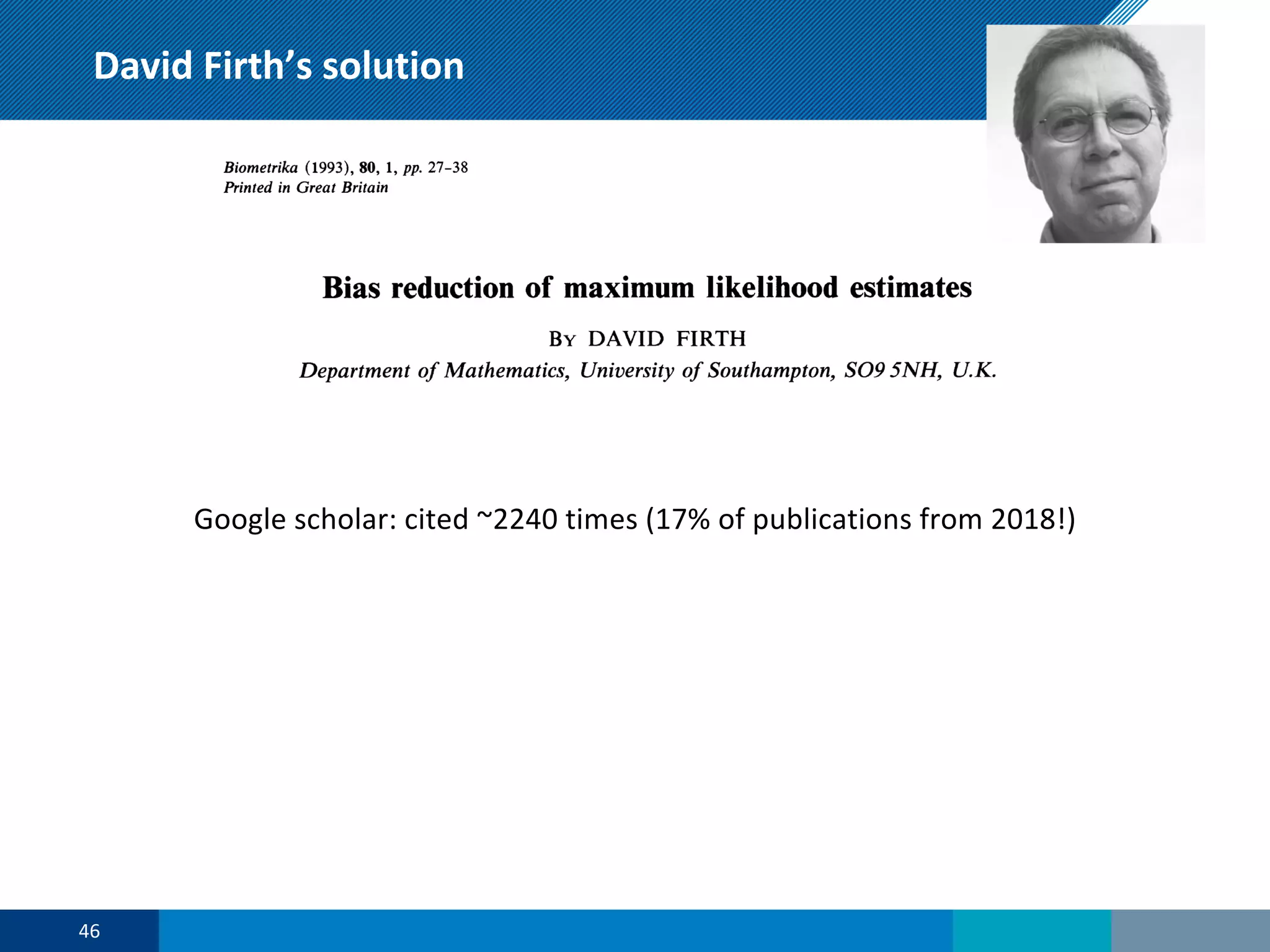
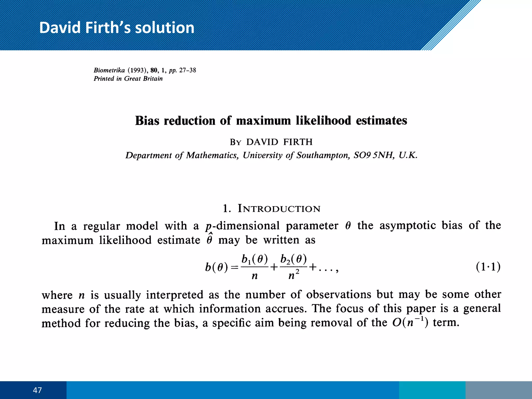
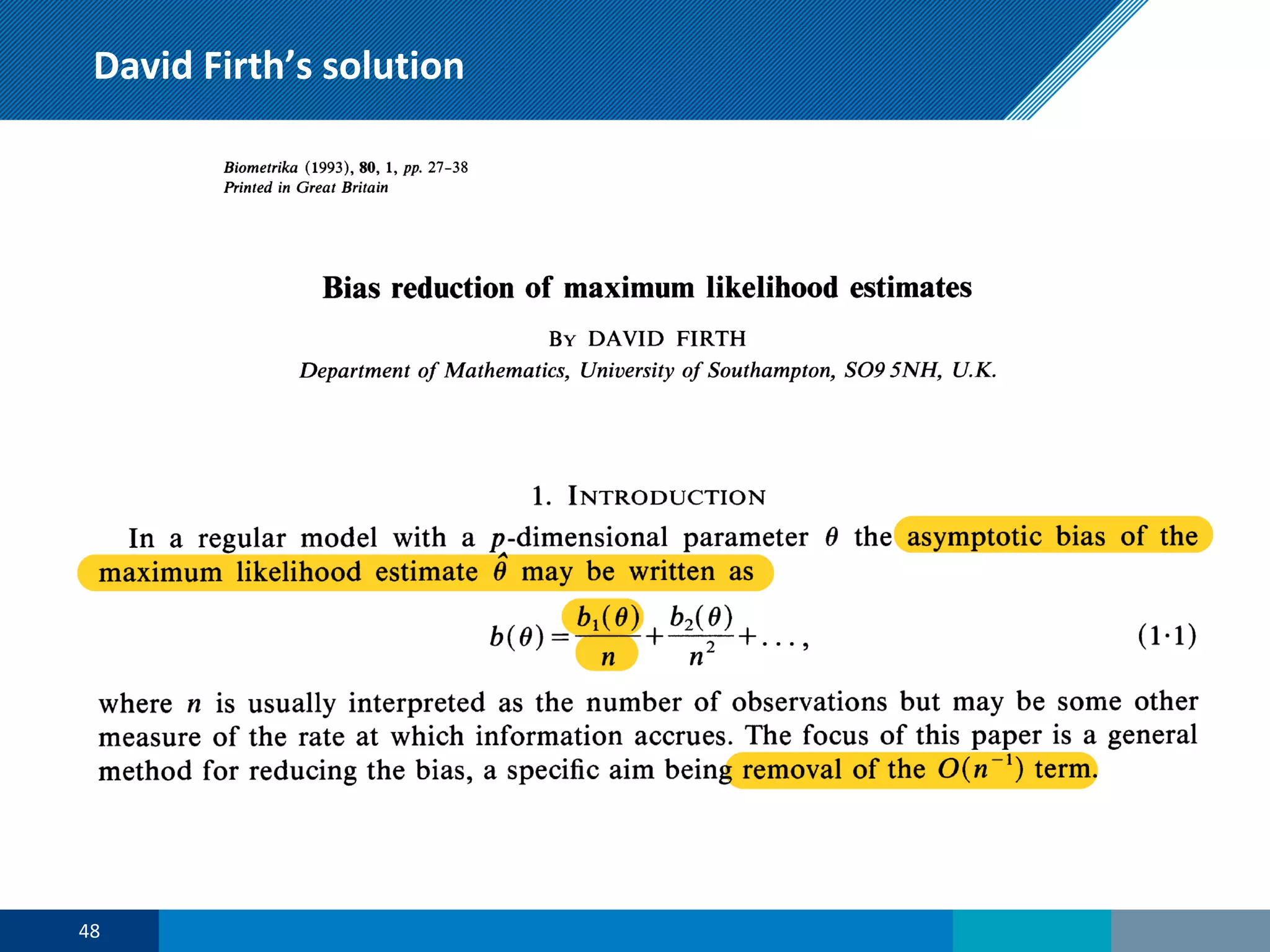
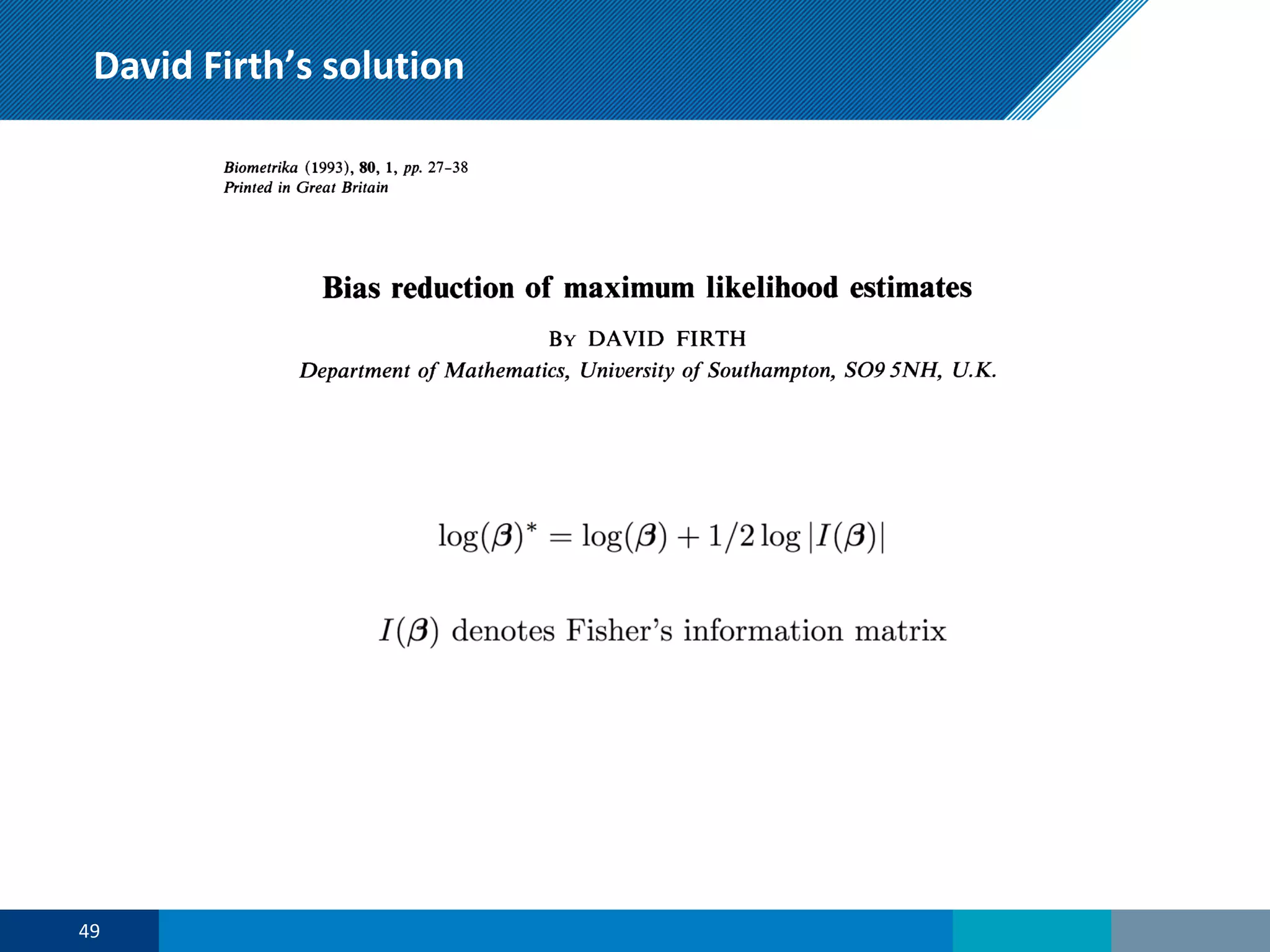
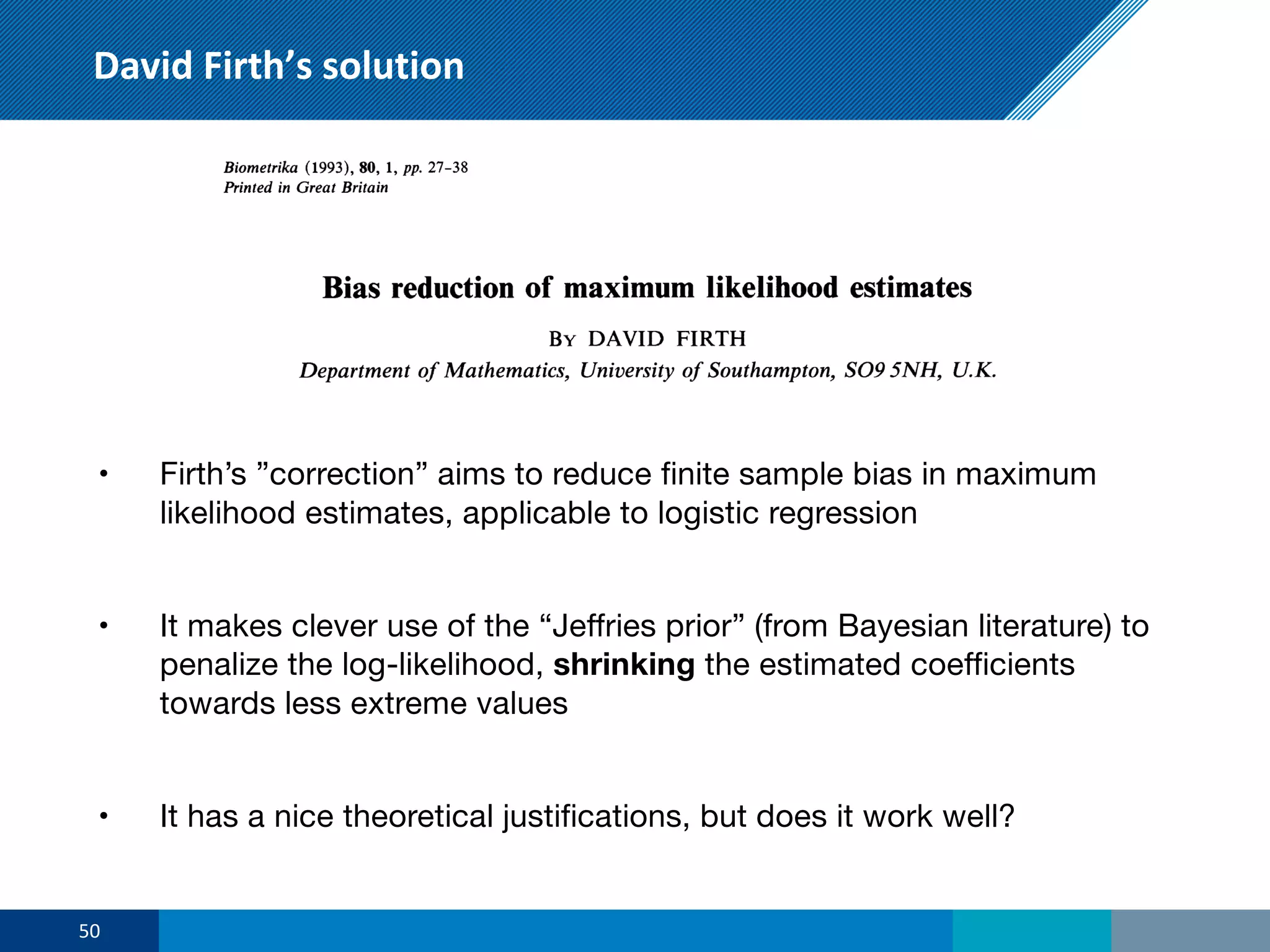
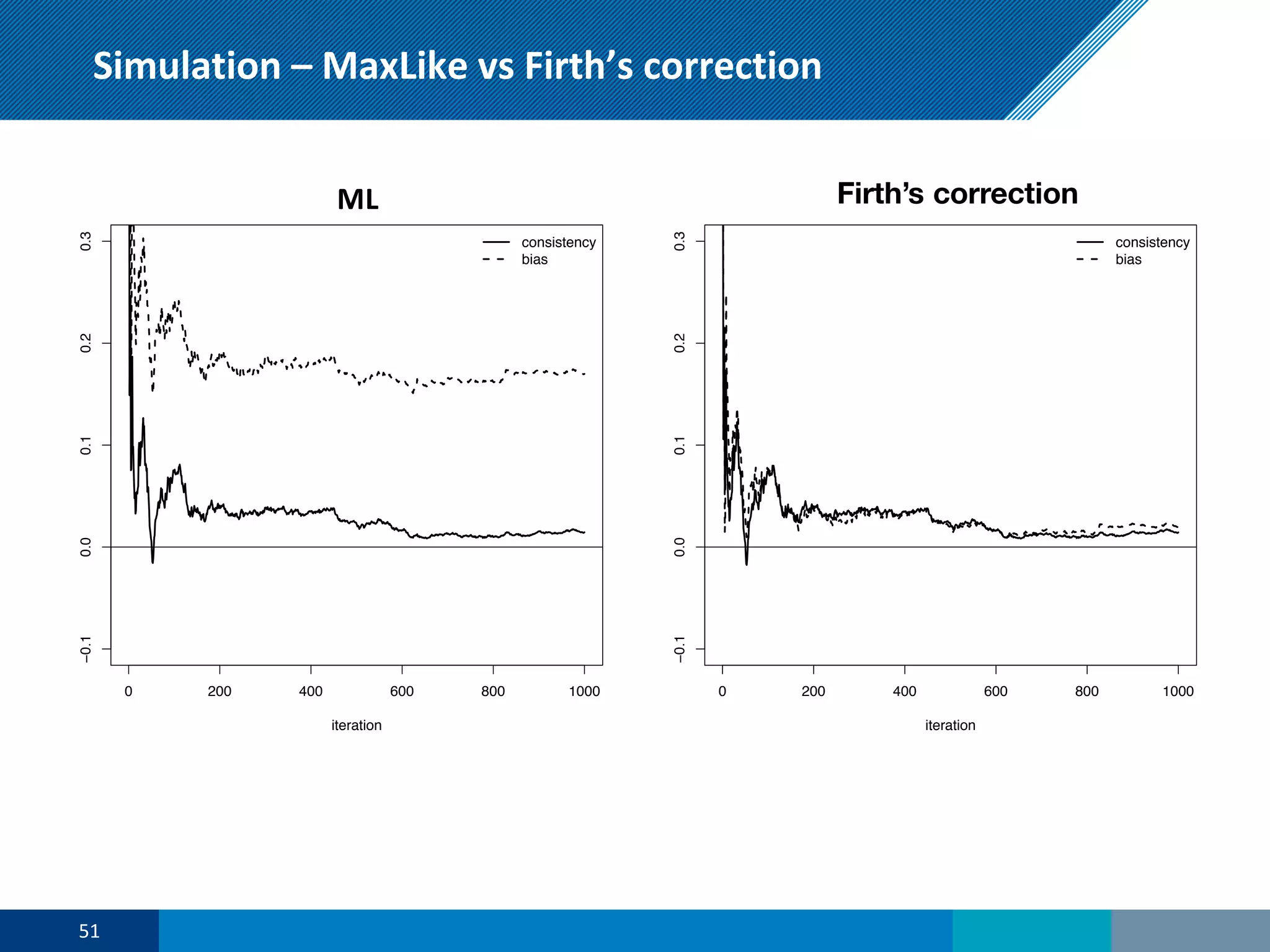
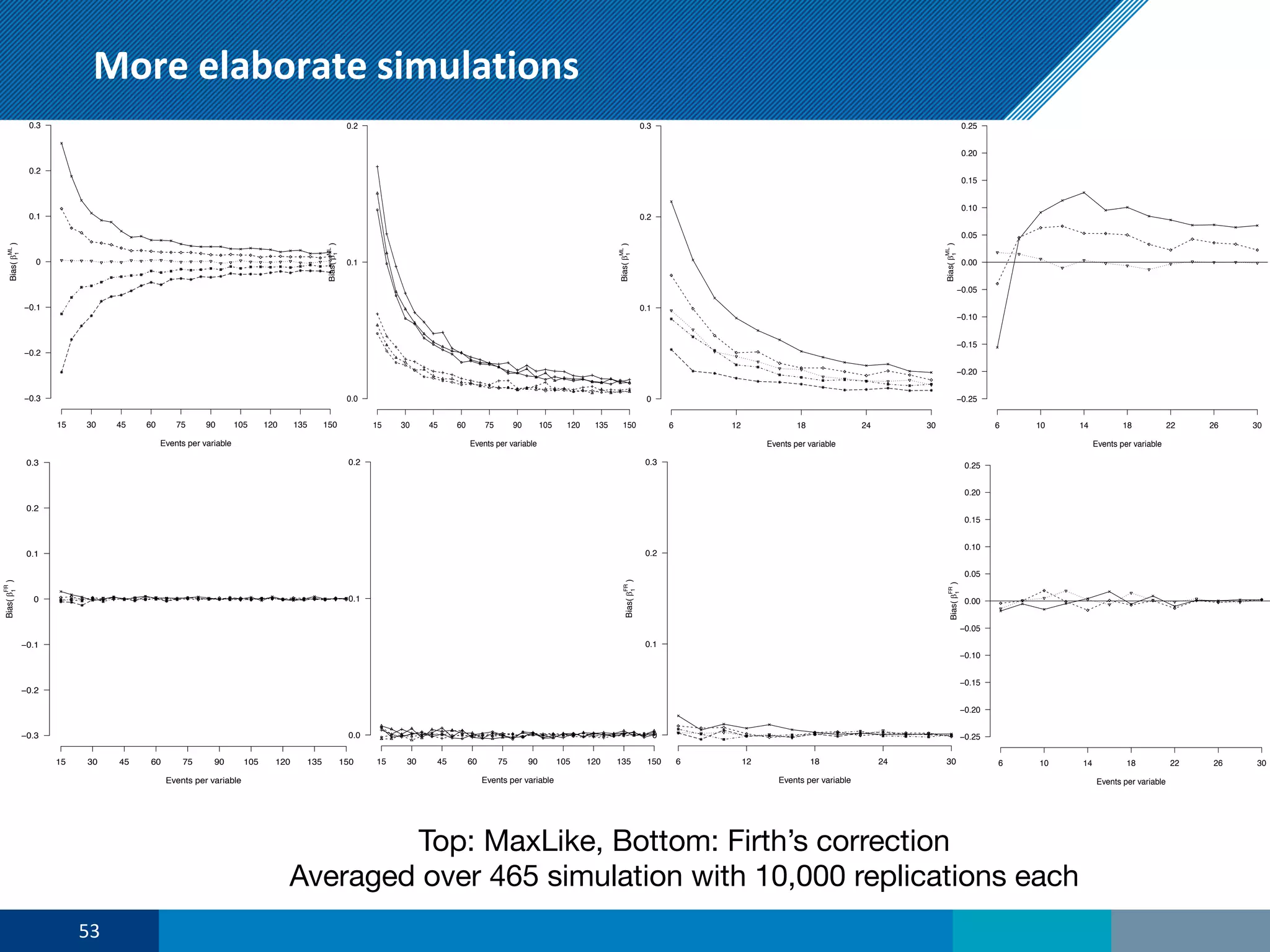
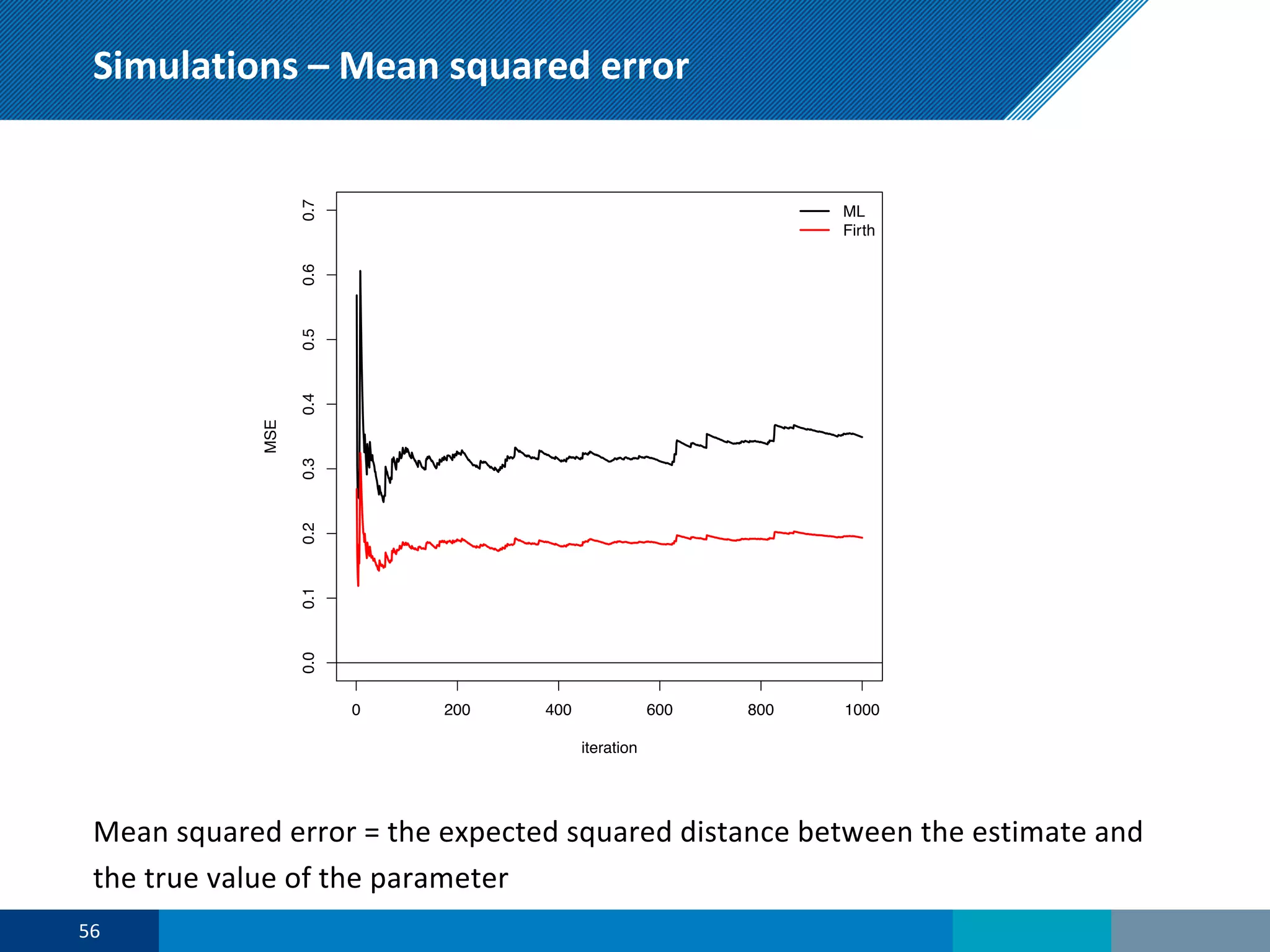
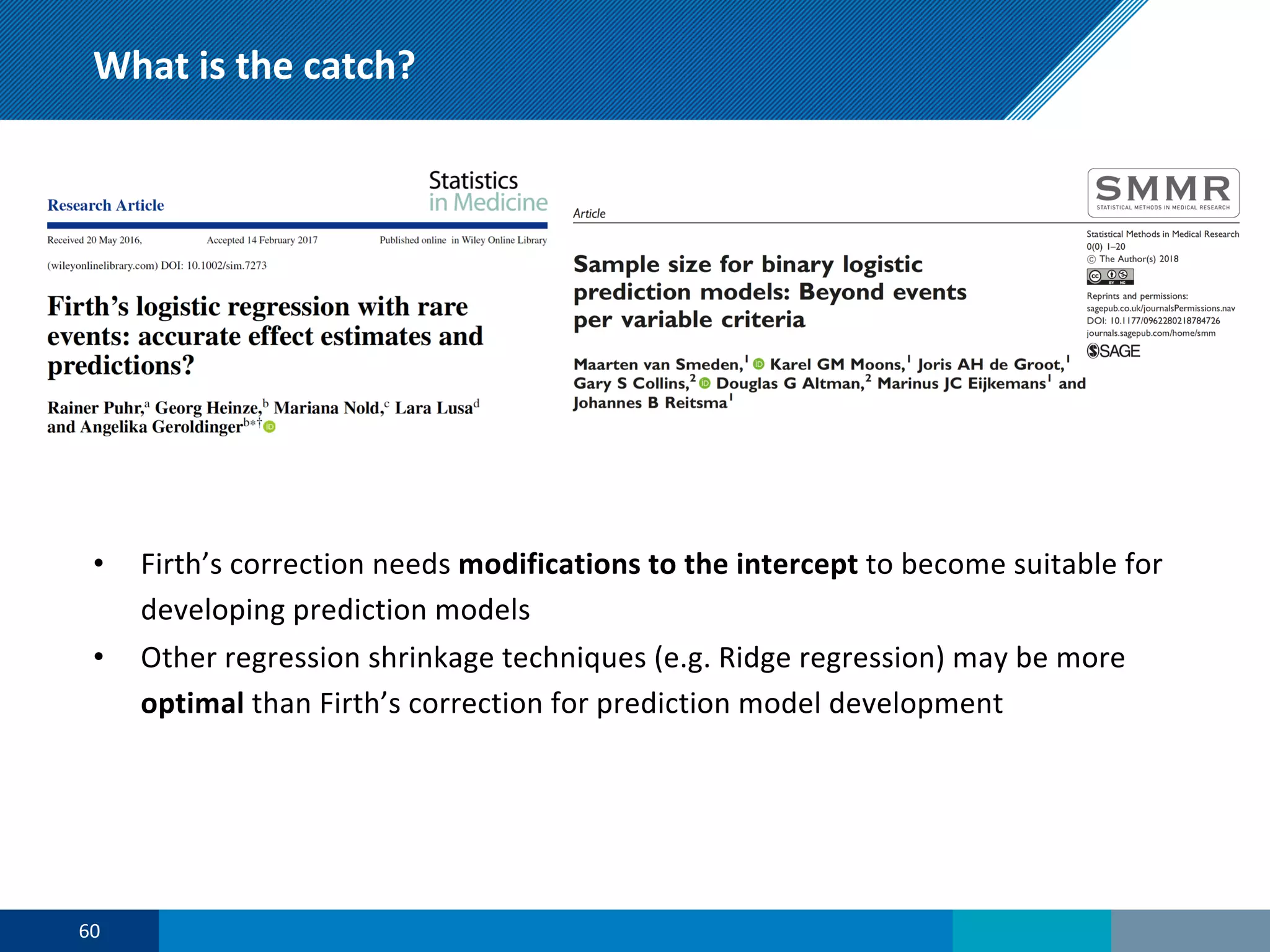
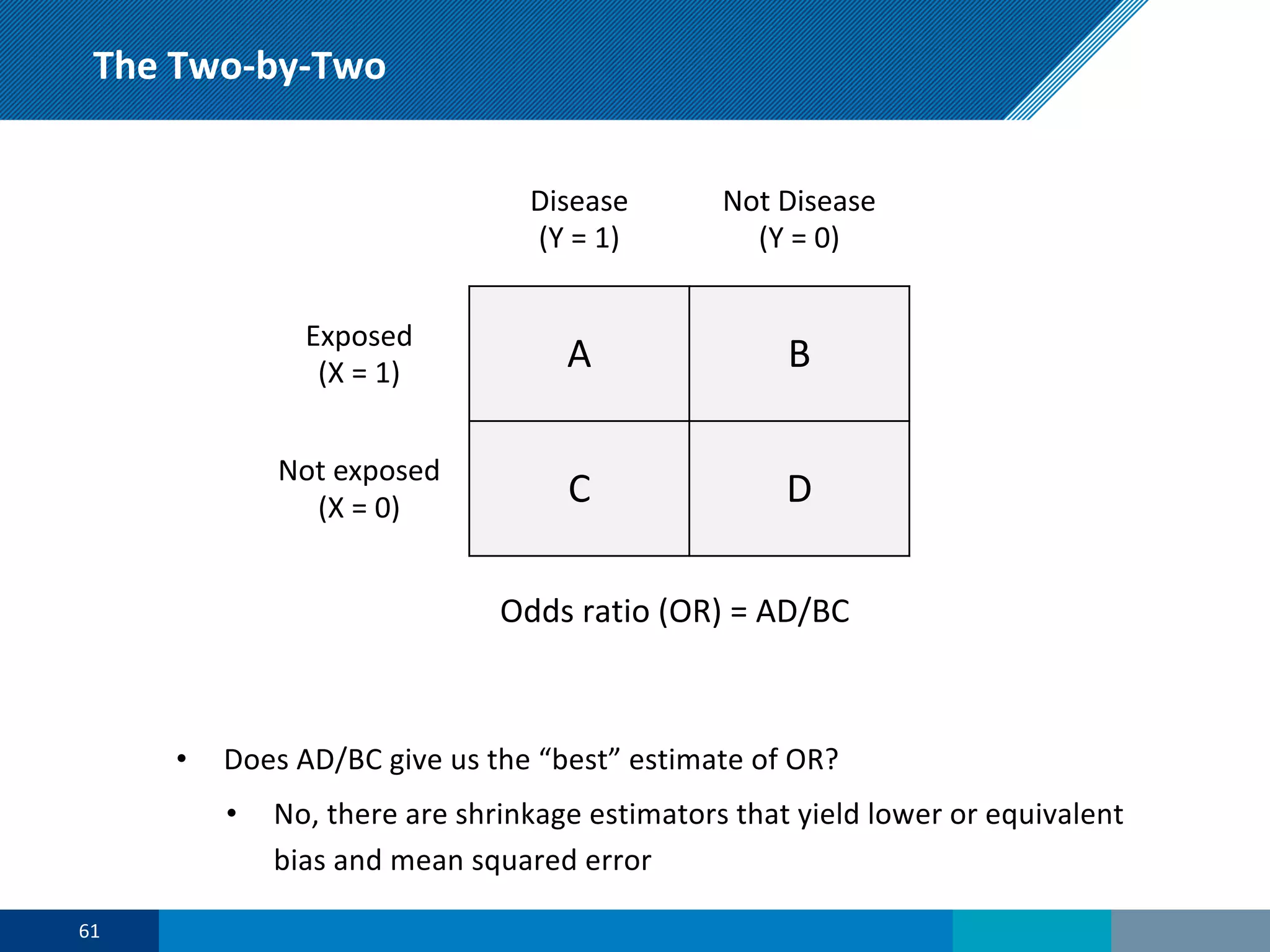
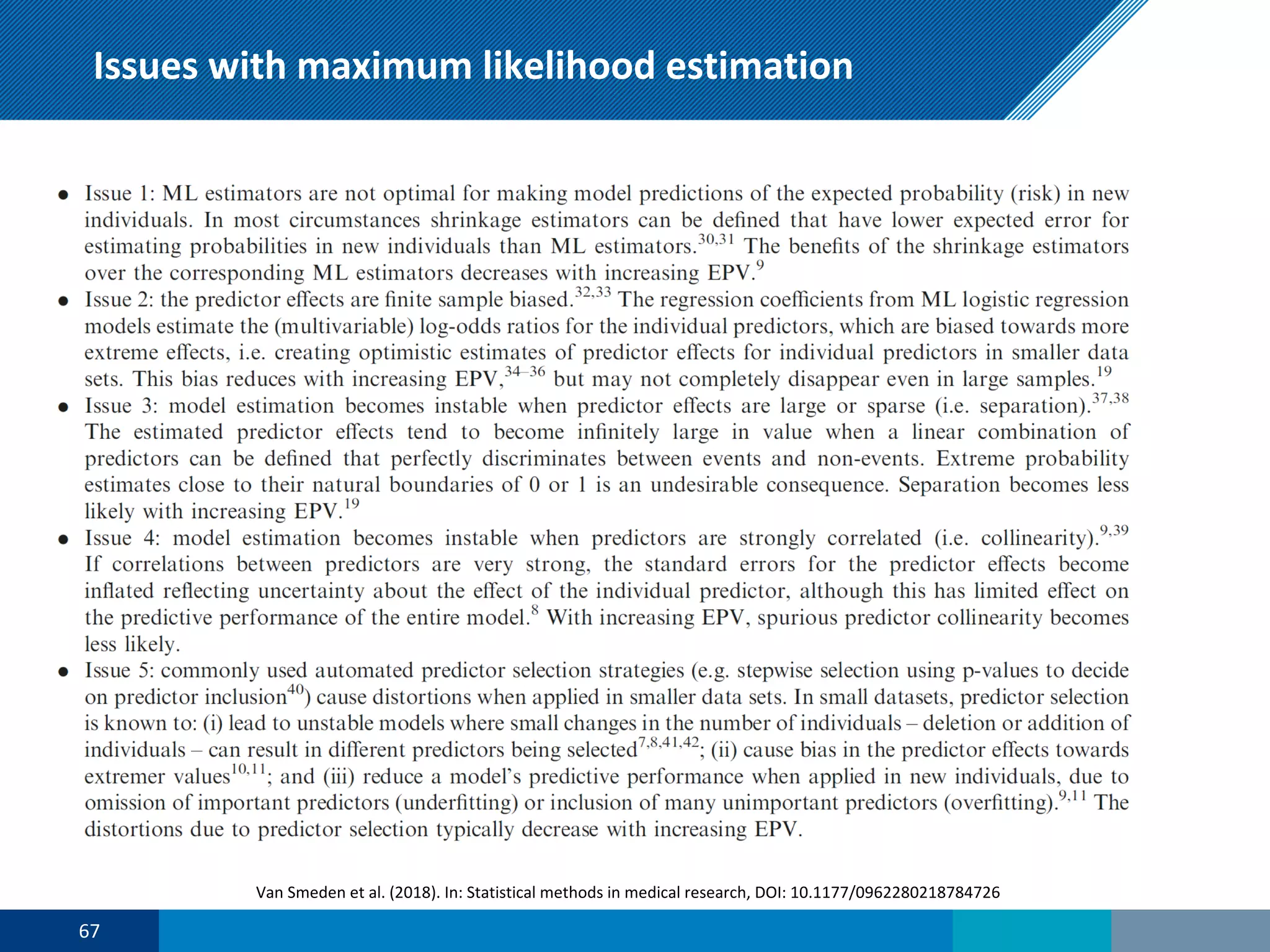
Berlin Epidemiological Methods Colloquium
Regression shrinkage:
better answers to causal questions
Dr Maarten van Smeden, Department of Clinical Epidemiology,
Leiden University Medical Center, Leiden, Netherlands
The slides of this talk
Go to: slideshare.net/MaartenvanSmeden/presentations
COI
No financial conflict of interest
Intellectual conflicts of interest
• I am convinced that the scientific discipline of epidemiologic research can have a
tremendous benefit to society if (and only if) research is done well
• It is my view that to maximise the benefit to society epidemiologic research needs to
be conducted while maintaining the highest standards of methodological rigor
• It is my view that epidemiologic research often does not benefit society due to,
among other reasons, a lack methodological rigor
• I am convinced that the methods topic of today is undervalued; better appreciation
has the potential to improve epidemiological analyses of almost any kind
• I have researched and published papers on today’s topic. I might overestimate the
importance of the methodological topic of today.
3
If you would be a real seeker after truth, it
is necessary that at least once in your life
you doubt, as far as possible, all things.
René Descartes (1644). Principles of Philosophy
4
Odds ratio (OR) = AD/BC
5
Disease
(Y = 1)
Not Disease
(Y = 0)
Exposed
(X = 1) A B
Not exposed
(X = 0) C D
• Does AD/BC give us the “best” estimate of OR?
• What is “best” anyway?
The Two-by-Two
This talk
Alternative approaches (estimators) for OR are generally ”better”
• By extension: default logistic regression output isn’t generally “best”
• Also true for default Cox models (and many other models)
Implications for causal inference oriented epidemiologic research
Better alternatives statistical models are widely implemented in software
6
To explain or to predict?
Explanatory models
• Theory: interest in regression coefficients
• Testing and comparing existing causal theories
• e.g. aetiology of illness, effect of treatment
Predictive models
• Interest in (risk) predictions of future observations
• No concern about causality
• Concerns about overfitting and optimism
• e.g. prognostic or diagnostic prediction model
Descriptive models
• Capture the data structure
7
Shmueli, G. (2010). To explain or to predict?. Statistical science, 25(3), 289-310.
Prof dr Galit Shmueli
To explain or to predict?
Explanatory models
• Theory: interest in regression coefficients
• Testing and comparing existing causal theories
• e.g. aetiology of illness, effect of treatment
Predictive models
• Interest in (risk) predictions of future observations
• No concern about causality
• Concerns about overfitting
• e.g. prognostic or diagnostic prediction model
Descriptive models
• Capture the data structure
8
Shmueli, G. (2010). To explain or to predict?. Statistical science, 25(3), 289-310.
Prof dr Galit Shmueli
1961
James and Stein. Estimation with quadratic loss. Proceedings of the fourth Berkeley symposium on mathematical statistics and probability. Vol. 1. 1961.
10
1977
Efron and Morris (1977). Stein′s paradox in statistics. Scientific American, 236 (5): 119–127.
11
1977
Efron and Morris (1977). Steinʹs paradox in statistics. Scientific American, 236 (5): 119–127.
12
Second half of the season
Efron and Morris (1977). Steinʹs paradox in statistics. Scientific American, 236 (5): 119–127.
Squared prediction
error
0.077
0.022
13
14
Shrinkage and overfitting (prediction)
Overfitting of prediction models
Model predictions of the expected probability (risk) in newindividuals too
extreme. By regression shrinkage the expected risks become less extreme
15
Shrinkage and overfitting (prediction)
Overfitting of prediction models:
Model predictions of the expected probability (risk) in newindividuals too
extreme. By regression shrinkage the expected risks become less extreme
16
Shrinkage for prediction literature (small selection)
17
To explain or to predict?
Explanatory models
• Theory: interest in regression coefficients
• Testing and comparing existing causal theories
• e.g. aetiology of illness, effect of treatment
Predictive models
• Interest in (risk) predictions of future observations
• No concern about causality
• Concerns about overfitting and optimism
• e.g. prognostic or diagnostic prediction model
Descriptive models
• Capture the data structure
18
Shmueli, G. (2010). To explain or to predict?. Statistical science, 25(3), 289-310.
A
L
Y
exposure outcome
confounder
Thinking about regression coefficient “wrongness”
19
Source: Yarkoni and Westfall (2017). In: Perspectives on Psychological Science, DOI: 10.1177/1745691617693393
Consider the simple(st) situation:
Binary logistic regression (binary outcome, 1 exposure, P-1 confounders)
Assumptions are (met):
1. Linear effects (in logit) and no interactions
2. ‘Low dimensional’: N >> P
3. IID sample (i.e., no clustering/nesting/matching/….)
4. No estimation issues (i.e., no co-linearity/separation/….)
5. Data complete: no missing values
6. No outliers
7. Data not very sparse (e.g. outcome events are not extremely rare)
8. No data-driven variable selection (DAG predefined)
9. Not any of the traditional sources of bias (confounding/information/selection)
24
Sources of bias
25
Epidemiology text-books
• Confounding bias
• Information bias
• Selection bias
Sources of bias
26
Epidemiology text-books
• Confounding bias: omit “common cause” L
• Information bias
• Selection bias
A
L
Y
exposure outcome
confounder
Sources of bias
27
Epidemiology text-books
• Confounding bias
• Information bias: e.g. measurement error in exposure
• Selection bias
A*
L
Y
true
exposure
outcome
confounder
measured
exposure
A
Sources of bias
28
Epidemiology text-books
• Confounding bias
• Information bias
• Selection bias: e.g. (not) lost to follow-up
A
L
Y
exposure outcome
confounder
C
Question
Which setting is likely to give the least amount of bias in the OR:
I. (average of) 100 studies of sample size 50
II. (average of) 10 studies of sample size 500
a) I & II: OR is unbiased
b) I & II: same amount of bias
c) I likely more bias than II
d) II likely more bias than I
29
Assume absence of:
• Confounding bias
• Information bias
• Selection bias
Statistical models
Binary Y, logistic regression
Pr Y = 1 a, l) = *+ = 1/ 1 + exp −lp+
Conditional effect of exposure, 234 in:
lp+ = 256 + 257a+ + 258l+(+ other confounders)
Exp(2β7): Multivariable odds ratio of the exposure effect (= OR of interest)
Likelihood
@ A = B
+
y+ log *+ + 1 − y+ log 1 − *+
30
..
A
L
Y
exposure outcome
confounder
Bias vs consistency
Unbiased estimator
In words: unbiased estimator = the expected value (think: large number of
replications) of the estimate equals the true value of the parameter
Consistent estimator
In words: consistency of estimator = as the sample size gets larger, the estimate
gets closer (in probability) to the true value of the parameter
31
log(OR): consistent but not unbiased
32
log(OR): consistent but not unbiased
33
Formal proof given in
Richardson comment in Stat Med (1985) that this proof was preceded by the same proof in Anderson and Richardson, 1979, Techometrics
34
Informal proof
• Simulate 1 exposure and 3 confounders
• Exposure and confounders related to outcome with equal multivariable odds-
ratios of 2.
• 1,000 simulation samples of N = 50
• Consistency: create 1,000 meta-dataset of increasing size: meta-dataset r
consists of each created dataset up to r;
Outcome: difference between meta-data estimates of exposure effect and
true value (log(OR) = log(2))
• Bias: calculate difference estimate of exposure effect and true value for each
of the created datasets up to r;
Outcome: difference between average of exposure effect estimates and true
value (log(OR) = log(2))
35
Simulation - result
0 200 400 600 800 1000
−0.10.00.10.20.3
iteration
consistency
36
0 200 400 600 800 1000
−0.10.00.10.20.3
iteration
●
consistency
~2% overestimated at N = 50,000
Simulation - result
37
Simulation - result
0 200 400 600 800 1000
−0.10.00.10.20.3
iteration
●
●
consistency
bias
~2% overestimated at N = 50,000
38
Simulation - result
0 200 400 600 800 1000
−0.10.00.10.20.3
iteration
●
●
consistency
bias
~2% overestimated at N = 50,000
~25% overestimated at (N = 50, 1000 replications)
39
Simulation - summary
• The magnitude of bias in exposure effect estimator (on the log odds scale) was
about 25% -> when evaluated on the odds ratio scale: bias is about 50%
• It is surprisingly easy to simulate situations that yield much larger bias (and
much smaller)
• The magnitude of bias depends on the sample size: “finite sample bias”
• Also:
• Number of confounders
• The size of the smallest outcome group (i.e. the event fraction)
• The distribution of the confounders and exposure
• The (true) effect sizes of confounders and exposure.
40
Sampling distribution
41
Van Smeden et al. (2016). In: BMC Medical research methodology, DOI: 10.1186/s12874-016-0267-3
Sampling distribution
42
Van Smeden et al. (2016). In: BMC Medical research methodology, DOI: 10.1186/s12874-016-0267-3
Implication
43
How we usually think about sample size
44
The implication of finite sample bias
45
David Firth’s solution
Google scholar: cited ~2240 times (17% of publications from 2018!)
46
David Firth’s solution
47
David Firth’s solution
48
David Firth’s solution
49
David Firth’s solution
• Firth’s ”correction” aims to reduce finite sample bias in maximum
likelihood estimates, applicable to logistic regression
• It makes clever use of the “Jeffries prior” (from Bayesian literature) to
penalize the log-likelihood, shrinking the estimated coefficients
towards less extreme values
• It has a nice theoretical justifications, but does it work well?
50
0 200 400 600 800 1000
−0.10.00.10.20.3
iteration
consistency
bias
Simulation – MaxLike vs Firth’s correction
ML
0 200 400 600 800 1000
−0.10.00.10.20.3
iteration
consistency
bias
Firth’s correction
Estimated bias reduced from ~25% with Maximum likelihood to ~ 3% with Firth’s correction.
51
More elaborate simulations
52
More elaborate simulations
Events per variable
Bias(b1
ML
)
15 30 45 60 75 90 105 120 135 150
−0.3
−0.2
−0.1
0
0.1
0.2
0.3
Events per variable
Bias(b1
ML
)
15 30 45 60 75 90 105 120 135 150
0.0
0.1
0.2
●
●
●
●
●
●
●
●
●
●
●
● ●
●
● ●
● ●
●
●
●
●
●
● ●
●
●
●
●
●
●
●
●
●
●
●
●
● ● ● ●
● ●
●
● ●
● ● ● ● ● ●
● ● ●
●
Events per variable
Bias(b1
ML
)
6 12 18 24 30
0
0.1
0.2
0.3
Events per variable
Bias(b1
ML
)
6 10 14 18 22 26 30
−0.25
−0.20
−0.15
−0.10
−0.05
0.00
0.05
0.10
0.15
0.20
0.25
Events per variable
Bias(b1
FR
)
15 30 45 60 75 90 105 120 135 150
0.0
0.1
0.2
●
● ●
●
●
●
●
● ●
●
●
●
●
●
● ●
● ●
● ●
●
● ●
●
●
●
●
●
●
● ●
●
● ● ● ● ● ● ● ● ● ●
● ● ● ● ● ● ● ●
●
● ●
● ● ●
Events per variable
Bias(b1
FR
)
6 12 18 24 30
0
0.1
0.2
0.3
Events per variable
Bias(b1
FR
)
6 10 14 18 22 26 30
−0.25
−0.20
−0.15
−0.10
−0.05
0.00
0.05
0.10
0.15
0.20
0.25
Top: MaxLike, Bottom: Firth’s correction
Averaged over 465 simulation with 10,000 replications each
53
Events per variable
Bias(b1
FR
)
15 30 45 60 75 90 105 120 135 150
−0.3
−0.2
−0.1
0
0.1
0.2
0.3
Three-line R analysis
> require(“logistf”)
> df <- read.csv(“mydata.csv”)
> logistf(Y~X1+X2+X3+X4, firth=T, data=df)
Numerical example (data were simulated)
logistf(formula = Y ~ X1 + X2 + X3 + X4, data = df, firth = T)
coef se(coef) lb.95 ub.95 Chisq p
(Intercept) 0.0405 0.3547 -0.6506 0.7267 0.0137 0.9067
X1 1.4319 0.5218 0.5160 2.5844 10.2622 0.0013
X2 0.6193 0.4502 -0.1924 1.5789 2.1967 0.1383
X3 0.8659 0.4036 0.1605 1.7738 6.0391 0.0139
X4 -0.6336 0.3770 - 1.4677 0.0331 3.4435 0.0635
Likelihood ratio test=20.53 on 4 df, p=0.0004, n=50
54
Other properties of Firth’s correction
Compared to maximum likelihood, Firth’s correction:
• Reduces both bias and mean squared error of the effect estimator
55
Simulations – Mean squared error
Mean squared error = the expected squared distance between the estimate and
the true value of the parameter
0 200 400 600 800 1000
0.00.10.20.30.40.50.60.7
iteration
MSE
ML
Firth
56
Other properties of Firth’s correction
Compared to maximum likelihood, Firth’s correction:
• Reduces both bias and mean squared error of the effect estimator
• Typically comes with smaller standard errors (narrower confidence intervals)
• Easy to apply in R, Stata and SAS, without noticeable extra computing time
• It is large-sample equivalent: for larger samples the estimates will hardly differ
between Firth’s correction and maximum likelihood estimates
• It remains finite in case of “separation” (when maximum likelihood fails)
57
Example of separation
58
Example of separation
59
What is the catch?
• Firth’s correction needs modifications to the intercept to become suitable for
developing prediction models
• Other regression shrinkage techniques (e.g. Ridge regression) may be more
optimal than Firth’s correction for prediction model development
60
Odds ratio (OR) = AD/BC
61
Disease
(Y = 1)
Not Disease
(Y = 0)
Exposed
(X = 1) A B
Not exposed
(X = 0) C D
• Does AD/BC give us the “best” estimate of OR?
• No, there are shrinkage estimators that yield lower or equivalent
bias and mean squared error
The Two-by-Two
62
Concluding remarks
• Standard logistic regression that is based on maximum likelihood estimation
produces estimates that are finite sample biased. When uncorrected, over-
optimistic estimates of effect may be produced
• Firth’s correction is a penalized estimation procedure that shrinks the
coefficients, thereby removing a large part of the finite sample bias
• Firth’s correction is also available for other popular models, such as Cox
models, conditional logistic regression models, Poisson regression and
multinomial logistic regression models. These models also produce estimates
that are finite sample biased
• The use of other shrinkage estimators, such as Ridge or LASSO should not be
taken lightly when causal inference is concerned. These approaches are
designed to create bias in effect estimators, rather than resolve it
64
The handouts of this presentation are available via:
https://www.slideshare.net/MaartenvanSmeden
R code to rerun and expand the simulations presented are available via:
https://github.com/MvanSmeden/LRMbias
Unfamiliar with R? Learn the basics in just two hours via:
http://www.r-tutorial.nl/
66
Issues with maximum likelihood estimation
67
Van Smeden et al. (2018). In: Statistical methods in medical research, DOI: 10.1177/0962280218784726

Regression shrinkage: better answers to causal questions

  • 1.
    Berlin Epidemiological MethodsColloquium Regression shrinkage: better answers to causal questions Dr Maarten van Smeden, Department of Clinical Epidemiology, Leiden University Medical Center, Leiden, Netherlands
  • 2.
    The slides ofthis talk Go to: slideshare.net/MaartenvanSmeden/presentations
  • 3.
    COI No financial conflictof interest Intellectual conflicts of interest • I am convinced that the scientific discipline of epidemiologic research can have a tremendous benefit to society if (and only if) research is done well • It is my view that to maximise the benefit to society epidemiologic research needs to be conducted while maintaining the highest standards of methodological rigor • It is my view that epidemiologic research often does not benefit society due to, among other reasons, a lack methodological rigor • I am convinced that the methods topic of today is undervalued; better appreciation has the potential to improve epidemiological analyses of almost any kind • I have researched and published papers on today’s topic. I might overestimate the importance of the methodological topic of today. 3
  • 4.
    If you wouldbe a real seeker after truth, it is necessary that at least once in your life you doubt, as far as possible, all things. René Descartes (1644). Principles of Philosophy 4
  • 5.
    Odds ratio (OR)= AD/BC 5 Disease (Y = 1) Not Disease (Y = 0) Exposed (X = 1) A B Not exposed (X = 0) C D • Does AD/BC give us the “best” estimate of OR? • What is “best” anyway? The Two-by-Two
  • 6.
    This talk Alternative approaches(estimators) for OR are generally ”better” • By extension: default logistic regression output isn’t generally “best” • Also true for default Cox models (and many other models) Implications for causal inference oriented epidemiologic research Better alternatives statistical models are widely implemented in software 6
  • 7.
    To explain orto predict? Explanatory models • Theory: interest in regression coefficients • Testing and comparing existing causal theories • e.g. aetiology of illness, effect of treatment Predictive models • Interest in (risk) predictions of future observations • No concern about causality • Concerns about overfitting and optimism • e.g. prognostic or diagnostic prediction model Descriptive models • Capture the data structure 7 Shmueli, G. (2010). To explain or to predict?. Statistical science, 25(3), 289-310. Prof dr Galit Shmueli
  • 8.
    To explain orto predict? Explanatory models • Theory: interest in regression coefficients • Testing and comparing existing causal theories • e.g. aetiology of illness, effect of treatment Predictive models • Interest in (risk) predictions of future observations • No concern about causality • Concerns about overfitting • e.g. prognostic or diagnostic prediction model Descriptive models • Capture the data structure 8 Shmueli, G. (2010). To explain or to predict?. Statistical science, 25(3), 289-310. Prof dr Galit Shmueli
  • 9.
    1961 James and Stein.Estimation with quadratic loss. Proceedings of the fourth Berkeley symposium on mathematical statistics and probability. Vol. 1. 1961. 10
  • 10.
    1977 Efron and Morris(1977). Stein′s paradox in statistics. Scientific American, 236 (5): 119–127. 11
  • 11.
    1977 Efron and Morris(1977). Steinʹs paradox in statistics. Scientific American, 236 (5): 119–127. 12
  • 12.
    Second half ofthe season Efron and Morris (1977). Steinʹs paradox in statistics. Scientific American, 236 (5): 119–127. Squared prediction error 0.077 0.022 13
  • 13.
  • 14.
    Shrinkage and overfitting(prediction) Overfitting of prediction models Model predictions of the expected probability (risk) in newindividuals too extreme. By regression shrinkage the expected risks become less extreme 15
  • 15.
    Shrinkage and overfitting(prediction) Overfitting of prediction models: Model predictions of the expected probability (risk) in newindividuals too extreme. By regression shrinkage the expected risks become less extreme 16
  • 16.
    Shrinkage for predictionliterature (small selection) 17
  • 17.
    To explain orto predict? Explanatory models • Theory: interest in regression coefficients • Testing and comparing existing causal theories • e.g. aetiology of illness, effect of treatment Predictive models • Interest in (risk) predictions of future observations • No concern about causality • Concerns about overfitting and optimism • e.g. prognostic or diagnostic prediction model Descriptive models • Capture the data structure 18 Shmueli, G. (2010). To explain or to predict?. Statistical science, 25(3), 289-310. A L Y exposure outcome confounder
  • 18.
    Thinking about regressioncoefficient “wrongness” 19 Source: Yarkoni and Westfall (2017). In: Perspectives on Psychological Science, DOI: 10.1177/1745691617693393
  • 19.
    Consider the simple(st)situation: Binary logistic regression (binary outcome, 1 exposure, P-1 confounders) Assumptions are (met): 1. Linear effects (in logit) and no interactions 2. ‘Low dimensional’: N >> P 3. IID sample (i.e., no clustering/nesting/matching/….) 4. No estimation issues (i.e., no co-linearity/separation/….) 5. Data complete: no missing values 6. No outliers 7. Data not very sparse (e.g. outcome events are not extremely rare) 8. No data-driven variable selection (DAG predefined) 9. Not any of the traditional sources of bias (confounding/information/selection) 24
  • 20.
    Sources of bias 25 Epidemiologytext-books • Confounding bias • Information bias • Selection bias
  • 21.
    Sources of bias 26 Epidemiologytext-books • Confounding bias: omit “common cause” L • Information bias • Selection bias A L Y exposure outcome confounder
  • 22.
    Sources of bias 27 Epidemiologytext-books • Confounding bias • Information bias: e.g. measurement error in exposure • Selection bias A* L Y true exposure outcome confounder measured exposure A
  • 23.
    Sources of bias 28 Epidemiologytext-books • Confounding bias • Information bias • Selection bias: e.g. (not) lost to follow-up A L Y exposure outcome confounder C
  • 24.
    Question Which setting islikely to give the least amount of bias in the OR: I. (average of) 100 studies of sample size 50 II. (average of) 10 studies of sample size 500 a) I & II: OR is unbiased b) I & II: same amount of bias c) I likely more bias than II d) II likely more bias than I 29 Assume absence of: • Confounding bias • Information bias • Selection bias
  • 25.
    Statistical models Binary Y,logistic regression Pr Y = 1 a, l) = *+ = 1/ 1 + exp −lp+ Conditional effect of exposure, 234 in: lp+ = 256 + 257a+ + 258l+(+ other confounders) Exp(2β7): Multivariable odds ratio of the exposure effect (= OR of interest) Likelihood @ A = B + y+ log *+ + 1 − y+ log 1 − *+ 30 .. A L Y exposure outcome confounder
  • 26.
    Bias vs consistency Unbiasedestimator In words: unbiased estimator = the expected value (think: large number of replications) of the estimate equals the true value of the parameter Consistent estimator In words: consistency of estimator = as the sample size gets larger, the estimate gets closer (in probability) to the true value of the parameter 31
  • 27.
    log(OR): consistent butnot unbiased 32
  • 28.
    log(OR): consistent butnot unbiased 33
  • 29.
    Formal proof givenin Richardson comment in Stat Med (1985) that this proof was preceded by the same proof in Anderson and Richardson, 1979, Techometrics 34
  • 30.
    Informal proof • Simulate1 exposure and 3 confounders • Exposure and confounders related to outcome with equal multivariable odds- ratios of 2. • 1,000 simulation samples of N = 50 • Consistency: create 1,000 meta-dataset of increasing size: meta-dataset r consists of each created dataset up to r; Outcome: difference between meta-data estimates of exposure effect and true value (log(OR) = log(2)) • Bias: calculate difference estimate of exposure effect and true value for each of the created datasets up to r; Outcome: difference between average of exposure effect estimates and true value (log(OR) = log(2)) 35
  • 31.
    Simulation - result 0200 400 600 800 1000 −0.10.00.10.20.3 iteration consistency 36
  • 32.
    0 200 400600 800 1000 −0.10.00.10.20.3 iteration ● consistency ~2% overestimated at N = 50,000 Simulation - result 37
  • 33.
    Simulation - result 0200 400 600 800 1000 −0.10.00.10.20.3 iteration ● ● consistency bias ~2% overestimated at N = 50,000 38
  • 34.
    Simulation - result 0200 400 600 800 1000 −0.10.00.10.20.3 iteration ● ● consistency bias ~2% overestimated at N = 50,000 ~25% overestimated at (N = 50, 1000 replications) 39
  • 35.
    Simulation - summary •The magnitude of bias in exposure effect estimator (on the log odds scale) was about 25% -> when evaluated on the odds ratio scale: bias is about 50% • It is surprisingly easy to simulate situations that yield much larger bias (and much smaller) • The magnitude of bias depends on the sample size: “finite sample bias” • Also: • Number of confounders • The size of the smallest outcome group (i.e. the event fraction) • The distribution of the confounders and exposure • The (true) effect sizes of confounders and exposure. 40
  • 36.
    Sampling distribution 41 Van Smedenet al. (2016). In: BMC Medical research methodology, DOI: 10.1186/s12874-016-0267-3
  • 37.
    Sampling distribution 42 Van Smedenet al. (2016). In: BMC Medical research methodology, DOI: 10.1186/s12874-016-0267-3
  • 38.
  • 39.
    How we usuallythink about sample size 44
  • 40.
    The implication offinite sample bias 45
  • 41.
    David Firth’s solution Googlescholar: cited ~2240 times (17% of publications from 2018!) 46
  • 42.
  • 43.
  • 44.
  • 45.
    David Firth’s solution •Firth’s ”correction” aims to reduce finite sample bias in maximum likelihood estimates, applicable to logistic regression • It makes clever use of the “Jeffries prior” (from Bayesian literature) to penalize the log-likelihood, shrinking the estimated coefficients towards less extreme values • It has a nice theoretical justifications, but does it work well? 50
  • 46.
    0 200 400600 800 1000 −0.10.00.10.20.3 iteration consistency bias Simulation – MaxLike vs Firth’s correction ML 0 200 400 600 800 1000 −0.10.00.10.20.3 iteration consistency bias Firth’s correction Estimated bias reduced from ~25% with Maximum likelihood to ~ 3% with Firth’s correction. 51
  • 47.
  • 48.
    More elaborate simulations Eventsper variable Bias(b1 ML ) 15 30 45 60 75 90 105 120 135 150 −0.3 −0.2 −0.1 0 0.1 0.2 0.3 Events per variable Bias(b1 ML ) 15 30 45 60 75 90 105 120 135 150 0.0 0.1 0.2 ● ● ● ● ● ● ● ● ● ● ● ● ● ● ● ● ● ● ● ● ● ● ● ● ● ● ● ● ● ● ● ● ● ● ● ● ● ● ● ● ● ● ● ● ● ● ● ● ● ● ● ● ● ● ● ● Events per variable Bias(b1 ML ) 6 12 18 24 30 0 0.1 0.2 0.3 Events per variable Bias(b1 ML ) 6 10 14 18 22 26 30 −0.25 −0.20 −0.15 −0.10 −0.05 0.00 0.05 0.10 0.15 0.20 0.25 Events per variable Bias(b1 FR ) 15 30 45 60 75 90 105 120 135 150 0.0 0.1 0.2 ● ● ● ● ● ● ● ● ● ● ● ● ● ● ● ● ● ● ● ● ● ● ● ● ● ● ● ● ● ● ● ● ● ● ● ● ● ● ● ● ● ● ● ● ● ● ● ● ● ● ● ● ● ● ● ● Events per variable Bias(b1 FR ) 6 12 18 24 30 0 0.1 0.2 0.3 Events per variable Bias(b1 FR ) 6 10 14 18 22 26 30 −0.25 −0.20 −0.15 −0.10 −0.05 0.00 0.05 0.10 0.15 0.20 0.25 Top: MaxLike, Bottom: Firth’s correction Averaged over 465 simulation with 10,000 replications each 53 Events per variable Bias(b1 FR ) 15 30 45 60 75 90 105 120 135 150 −0.3 −0.2 −0.1 0 0.1 0.2 0.3
  • 49.
    Three-line R analysis >require(“logistf”) > df <- read.csv(“mydata.csv”) > logistf(Y~X1+X2+X3+X4, firth=T, data=df) Numerical example (data were simulated) logistf(formula = Y ~ X1 + X2 + X3 + X4, data = df, firth = T) coef se(coef) lb.95 ub.95 Chisq p (Intercept) 0.0405 0.3547 -0.6506 0.7267 0.0137 0.9067 X1 1.4319 0.5218 0.5160 2.5844 10.2622 0.0013 X2 0.6193 0.4502 -0.1924 1.5789 2.1967 0.1383 X3 0.8659 0.4036 0.1605 1.7738 6.0391 0.0139 X4 -0.6336 0.3770 - 1.4677 0.0331 3.4435 0.0635 Likelihood ratio test=20.53 on 4 df, p=0.0004, n=50 54
  • 50.
    Other properties ofFirth’s correction Compared to maximum likelihood, Firth’s correction: • Reduces both bias and mean squared error of the effect estimator 55
  • 51.
    Simulations – Meansquared error Mean squared error = the expected squared distance between the estimate and the true value of the parameter 0 200 400 600 800 1000 0.00.10.20.30.40.50.60.7 iteration MSE ML Firth 56
  • 52.
    Other properties ofFirth’s correction Compared to maximum likelihood, Firth’s correction: • Reduces both bias and mean squared error of the effect estimator • Typically comes with smaller standard errors (narrower confidence intervals) • Easy to apply in R, Stata and SAS, without noticeable extra computing time • It is large-sample equivalent: for larger samples the estimates will hardly differ between Firth’s correction and maximum likelihood estimates • It remains finite in case of “separation” (when maximum likelihood fails) 57
  • 53.
  • 54.
  • 55.
    What is thecatch? • Firth’s correction needs modifications to the intercept to become suitable for developing prediction models • Other regression shrinkage techniques (e.g. Ridge regression) may be more optimal than Firth’s correction for prediction model development 60
  • 56.
    Odds ratio (OR)= AD/BC 61 Disease (Y = 1) Not Disease (Y = 0) Exposed (X = 1) A B Not exposed (X = 0) C D • Does AD/BC give us the “best” estimate of OR? • No, there are shrinkage estimators that yield lower or equivalent bias and mean squared error The Two-by-Two
  • 57.
  • 59.
    Concluding remarks • Standardlogistic regression that is based on maximum likelihood estimation produces estimates that are finite sample biased. When uncorrected, over- optimistic estimates of effect may be produced • Firth’s correction is a penalized estimation procedure that shrinks the coefficients, thereby removing a large part of the finite sample bias • Firth’s correction is also available for other popular models, such as Cox models, conditional logistic regression models, Poisson regression and multinomial logistic regression models. These models also produce estimates that are finite sample biased • The use of other shrinkage estimators, such as Ridge or LASSO should not be taken lightly when causal inference is concerned. These approaches are designed to create bias in effect estimators, rather than resolve it 64
  • 60.
    The handouts ofthis presentation are available via: https://www.slideshare.net/MaartenvanSmeden R code to rerun and expand the simulations presented are available via: https://github.com/MvanSmeden/LRMbias Unfamiliar with R? Learn the basics in just two hours via: http://www.r-tutorial.nl/
  • 61.
  • 62.
    Issues with maximumlikelihood estimation 67 Van Smeden et al. (2018). In: Statistical methods in medical research, DOI: 10.1177/0962280218784726