Custom Writing Service http://StudyHub.vip/Anthropogenic-And-Natural-Causes-Of-Cli 👈

1. Anthropogenic and natural causes of climate change
David I. Stern & Robert K. Kaufmann
Received: 27 March 2013 /Accepted: 7 November 2013 /Published online: 20 November 2013
# Springer Science+Business Media Dordrecht 2013
Abstract We test for causality between radiative forcing and temperature using
multivariate time series models and Granger causality tests that are robust to the
non-stationary (trending) nature of global climate data. We find that both natural and
anthropogenic forcings cause temperature change and also that temperature causes
greenhouse gas concentration changes. Although the effects of greenhouse gases and
volcanic forcing are robust across model specifications, we cannot detect any effect
of black carbon on temperature, the effect of changes in solar irradiance is weak,
and the effect of anthropogenic sulfate aerosols may be only around half that
usually attributed to them.
1 Introduction
Despite a strengthening consensus that the increase in anthropogenic emissions of
greenhouse gases is partially responsible for the observed increase in global temper-
ature since the mid-20th century, scientific debate continues on several issues, includ-
ing the relative size of individual causes of climate change such as sulfate aerosols
(Kaufmann et al. 2011), the El Nino-Southern Oscillation (Compo and Sardeshmukh
2010; Tung and Zhou 2013), black carbon (Bond et al. 2013), the existence of climate
feedbacks on the global carbon cycle (Piao et al. 2008; Barichivich et al. 2012), and
whether increases in carbon dioxide precede or follow global warming (Shakun et al.
2012; Parrenin et al. 2013). Here, we test for causality between radiative forcing and
temperature using multivariate time series models and Granger causality tests that are
robust to the non-stationary (trending) nature of global climate data.
One approach to detecting and attributing climate change involves estimating time
series models of the relation between temperature and relevant forcing variables (e.g.
Stone and Allen 2005; Stern 2006; Lean and Rind 2008; Beenstock et al. 2012; Canty
et al. 2012). The validity of these models depends critically on the time series
properties of the variables and the model residuals (Stern and Kaufmann 2000).
Climatic Change (2014) 122:257–269
DOI 10.1007/s10584-013-1007-x
D. I. Stern (*)
Crawford School of Public Policy, Australian National University, Canberra, ACT 0200, Australia
e-mail: david.stern@anu.edu.au
R. K. Kaufmann
Department of Earth and Environment, Boston University, Boston, MA 02215, USA
e-mail: kaufmann@bu.edu

2. Specifically, the time series for many forcings are non-stationary, and may be sto-
chastically trending (Stern and Kaufmann 2000)—only the changes in the variable are
stationary—which invalidates the naive application of classical static regression anal-
ysis. However, it is very hard to identify the actual data generating process, and,
therefore, the statistical properties of the time series, because available tests have low
statistical power to discriminate among alternatives, and the temperature series, in
particular, are noisy due to internal variability (Stern and Kaufmann 2000).
Alternatively, robust Granger causality tests that do not depend on the statistical
properties of the time series (Toda and Yamamoto 1995) may offer a more reliable
approach to attributing climate change to specific forcings. A time series variable x
(e.g. radiative forcing) is said to Granger cause variable y (e.g. surface temperature) if
past values of x help predict the current level of y given all other relevant informa-
tion. This hypothesis can be tested by estimating a multivariate time series model,
known as a vector autoregression (VAR), for x, y, and other relevant variables. The
VAR models the current values of each variable as a linear function of their own past
values and those of the other variables. Then we test the hypothesis that x does not
cause y by evaluating restrictions that exclude the past values of x from the equation
for y and vice versa.
Granger causality tests depend on which additional variables are included or
excluded from the statistical model. If the model omits an important causal variable,
omitted variable bias can generate false conclusions about Granger causality
(Lütkepohl 1982). In particular, interpreting a finding that a variable Granger causes
another variable only implies actual causation if other possible causes are controlled
for (Granger 1988). Therefore, in this paper, we test the effects of potential forcings
while controlling for the effects of all other relevant forcings. The notion of Granger
causality depends on the ability of one variable to predict another conditional on other
relevant information. While rejection of the null that a variable does not help predict
the other while controlling for other relevant causes might reasonably be taken as an
indication of causation per se, non-rejection of the null could be due to a variety of
other reasons discussed in the next section of the paper. Therefore, we need to be
cautious in interpreting a finding of no Granger causality as implying that there is
truly no causal relationship between the variables.
To identify causal relations between radiative forcing and temperature and explore
uncertainty about the effects, we compile annual global time series data for temper-
ature and an expanded set of radiative forcings from 1850 to 2011, create several
scenarios for the relative size of uncertain forcings, and test for Granger causality
between the radiative forcing and temperature series using Toda and Yamamoto’s
(1995) robust Granger causality test. We find that both natural and anthropogenic
forcings cause temperature change and also that temperature causes greenhouse gas
concentrations.1
Additionally, though the effects of greenhouse gases and volcanic
forcing are robust across model specifications, we cannot detect any effect of black
carbon on temperature, the effect of changes in solar irradiance is weak, and the effect
of anthropogenic sulfate aerosols may be only around half that usually attributed to
them (Boucher and Pham 2002).
1
Here and in the remainder of the paper we use “cause” for “Granger cause” to make the paper more readable.
258 Climatic Change (2014) 122:257–269

3. 2 Statistical methods
To account for the effects of m control variables, zj, we expand the simple bi-variate model
used to test for causality between two variables, x and y, described above, by estimating the
following model:
xt ¼ α1 þ
X
i¼1
p
Πi
1;1
xt−i þ
X
i¼1
p
Πi
1;2
yt−i þ
X
j¼1
m X
i¼1
p
Πi
1;2þ j
zj;t−i þ ε1t ð1Þ
yt ¼ α2 þ
X
i¼1
p
Πi
2;1
xt−i þ
X
i¼1
p
Πi
2;2
yt−i þ
X
j¼1
m X
i¼1
p
Πi
2;2þ j
zj;t−i þ ε2t ð2Þ
zkt ¼ α2þj þ
X
i¼1
p
Πi
2þk;1
xt−i þ
X
i¼1
p
Πi
2þk;2
yt−i þ
X
j¼1
m X
i¼1
p
Πi
2þk;3
zjt−i þ ε2þkt; ∀k ¼ 1; …; m ð3Þ
where t indexes time and p is the number of lags that adequately models the dynamic structure
so that the coefficients of further lags of variables are not statistically significant. There are p
matrices of regression coefficients Πi
, which have dimension (2+m)×(2+m) and α is a (2+m)
vector of regression coefficients. The error terms ε are white noise though they may be
correlated across equations. The null hypothesis Π1
2;1
¼ Π2
2;1
¼ … ¼ Πp
2;1
¼ 0 implies that
x does not cause y. Rejecting this null indicates that x causes y. Similarly, rejecting
Π1
1;2
¼ Π2
1;2
¼ … ¼ Πp
1;2
¼ 0 indicates that y causes x.
Failure to reject the null hypothesis that x does not cause y, does not necessarily mean that
there is no causal relation between the variables. Instead, among other possibilities, a
misspecified number of lags of the variables, insufficiently frequent observations (Granger
1988), too small a sample and hence low statistical power, omitted variables bias (Lütkepohl
1982), nonlinearity (Sugihara et al. 2012), and model dynamics where the effects of different
casual channels cancel each other out (Jacobs et al. 1979) 2
can generate a type II error.
Regarding non-linearity, a linear VAR should be appropriate for testing for causality because
the response of the climate system to forcings appears to be linear and additive on large spatial
scales (Stone et al. 2009).
Toda and Yamamoto (1995) modify the standard Granger causality test on the variables in
levels so that their test of casuality is robust to the presence of integrated variables and non-
cointegration. Specifically, they add one additional lag of the variables to the standard VAR
model for each possible degree of integration. So if variables are integrated at most of order
one then one additional lag is added and if variables are possibly second order integrated (I(2))
2
Jacobs et al. (1979) propose a structural vector autoregression model where there are also simultaneous or
instantanteous interactions among the variables. They list three different hypotheses about the causality between
variables x and y. In the context of their hypotheses, non-rejection of the null hypothesis of non-casuality from x
to y in our equation (2) could be because there are neither instantaneous nor lagged effects of x on y – their H1.
But shocks to x in previous periods affect the current of value of y through both the direct effect of the lagged
value of x on y and through their effect on the current value of x and it is possible that these two effects exactly
cancel so that past values of x do not improve forecasts of y—their H3. They argue that non-rejection of the null
of no Granger causality does not mean that there is no actual causality. This situation is rather unlikely (Sargent
1979). Note, that if there are only instantaneous effects in their structural model, past values of x will be useful in
predicting y.
Climatic Change (2014) 122:257–269 259

4. two lags are added. These additional lags are not restricted in the Granger causality test. The test
statistic has the classic asymptotically chi-squared distribution with p degrees of freedom.
Hacker and Hatemi-J (2006) show that using a sample of 100 observations and two extra lags
generates results in which the null hypothesis is rejected at rates that are close to but slightly
larger than the significance levels given by the chi-squared distribution. The model estimated is:
yt ¼ α þ
X
i¼1
p
Πiyt−iþ
X
i¼1
d
Φiyt−p−iþεt ð4Þ
where y is now a vector of n variables, ε is a vector of n white noise error terms, d is the maximal
order of integration in the data, and t indexes time. We estimate the model using the seemingly
unrelated regressions estimator and impose the restrictions on the system of equations. We use the
Schwert criterion to fix the maximal lag length for the VAR models, which for the 1850–2011 and
1880–2011 samples is 4 lags, and for the 1958–2011 sample is 3 lags. We use the Schwarz
Bayesian Information Criterion (SBC) to determine the optimal lag length (Schwarz 1978). Table 1
presents the optimal lag lengths for the various model set-ups and variable definitions. We set d=2
as previous studies (Stern and Kaufmann 2000; Beenstock et al. 2012) find that some variables
might be I(2). To reduce the number of parameters that are estimated, we impose exogeneity
restrictions on the aerosol and solar irradiance variables in the disaggregated version of the model.
3 Data sources and calculation of radiative forcing
Temperature We use two global land-sea temperature series—HADCRUT4 (Morice et al.
2012) and GISS v3 GLOBAL Land-Ocean Temperature Index (Hansen et al. 2010). GISS data
are only available from 1880 while HADCRUT4 are available from 1850.
Ocean heat content We obtain data from:
http://www.nodc.noaa.gov/OC5/3M_HEAT_CONTENT/basin_data.html
We use the 0–700 m layer series, as only these data are available with unsmoothed annual
observations. Data is available from 1955 to 2011. See Levitus et al. (2012) for more details.
Radiative forcing We update to 2011 the sources used in Stern (2006) with the following
modifications:
Volcanic sulfate aerosol: We use the optical thickness data from GISS:
http://data.giss.nasa.gov/modelforce/strataer/tau_line.txt
Radiative forcing is −27 times the optical thickness. See Sato et al. (1993) for discussion of
sources and methods.
Anthropogenic sulfur emissions: We use data from Smith et al. (2011) and Klimont et al. (2013).
Radiative forcing is computed using a modification of the formula in Wigley and Raper (1992) and
values from Boucher and Pham (2002) of −0.42Wm−2
for direct radiative forcing in 1990 and
−1.0Wm−2
for indirect forcing in 1990, an indirect forcing of −0.17Wm−2
in 1850, and a natural
burden of 0.19Tg S and an anthropogenic burden of 0.47 Tg S in 1990. The formula for indirect
forcing is:
Rt ¼ −0:13−0:87ln 1 þ htSt
.
26
.
ln 1 þ htS1990
.
26
ð5Þ
where S is annual anthropogenic sulfur emissions in Tg S and h is the stack height term (Wigley and
Raper 1992).
260 Climatic Change (2014) 122:257–269

5. Table 1 Selection of the optimal lag length
Data set HADCRUT4
Sample 1850–2011 1958–2011
Ocean heat content No No Yes
Alternative Scenarios BC=1 BC=0 BC=3 BC=0 S=0.5 BC=1 BC=0 BC=3 BC=0 S=0.5 BC=1 BC=0 BC=3 BC=0 S=0.5
Forcing variables:
RFTOT 1 1 1 1 2 2 2 1 1 1 1 1
RFANTH RFNAT 2 2 2 2 2 2 2 2 1 1 1 1
RFGHG RFSOX RFBC RFSOL RFVOL 2 1 1
Data set GISS3
Sample 1850–2011 1958–2011
Ocean Heat Content No No Yes
Alternative Scenarios BC=1 BC=0 BC=3 BC=0 S=0.5 BC=1 BC=0 BC=3 BC=0 S=0.5 BC=1 BC=0 BC=3 BC=0 S=0.5
Forcing variables:
RFTOT 1 1 1 1 2 2 2 2 1 1 1 1
RFANTH RFNAT 2 2 1 2 2 2 2 2 1 1 1 1
RFGHG RFSOX RFBC RFSOL RFVOL 2 1 1
Figures are number of lags chosen
Climatic
Change
(2014)
122:257–269
261

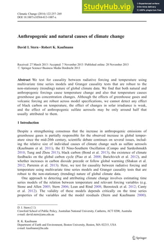
6. Black and organic carbon: We use the radiative forcing provided in RCP 8.5 (Meinshausen
et al. 2011). We sum the variables OCI_RF, BCI_RF, BIOMASSAER_RF, and BCSNOW_RF
to get the total effect of black and organic carbon.
It is possible to adjust the temperature series for the effects of ENSO and other oscillations.
Several adjusted time series are available, but they are only weakly correlated, especially in
earlier years and some of these reconstructions (e.g. Compo and Sardeshmukh 2010; Tung and
Zhou 2013) remove much of the variance in the temperature series. However, these oscilla-
tions are an endogenous part of the climate system, which might be affected by anthropogenic
and natural forcing and, therefore, their effects should not necessarily be removed from the
temperature data.
4 Results
We use alternative scenarios for the relative size of the forcings to explore the considerable
uncertainty regarding the effects of black carbon and anthropogenic sulfate emissions (Forster
et al. 2007). Bond et al. (2013) find that the radiative forcing due to black carbon is likely to be
much greater than previously estimated. However, this new estimate has a wide confidence
interval that also includes zero. We investigate this uncertainty by evaluating scenarios for a
range of values for the radiative forcing of black carbon and sulfate aerosols. The standard
scenario (indicated as BC=1, S=1) assumes that the radiative forcing of black carbon and
anthropogenic sulfate aerosols in 1990 is 0.31 Wm−2
(Meinshausen et al. 2011) and −1.42
Wm−2
(Boucher and Pham 2002), respectively.
Based on these values, anthropogenic forcing (greenhouse gases, sulfur emissions, and
black carbon) is low until 1970 after which it increases sharply (Fig. 1a). Natural forcings are
dominated by large volcanic eruptions (Fig. 1b). In the last decade, total anthropogenic and
natural forcing is fairly constant due to a decline in natural forcing and a slight slowing in the
growth of the anthropogenic forcing. This might partly explain the relative hiatus in global
temperature increase in this period (Kaufmann et al. 2011). Similarly, both atmospheric
temperature and ocean heat content show an increase starting around 1970 and a slowing
during the last decade (Fig. 2). Alternative scenarios (BC=0, S=1 and BC=3, S=1) assume
that black carbon either makes no contribution to global warming or has three times the
standard effect, or (BC=0, S=0.5) assumes that black carbon has no effect and anthropogenic
sulfate aerosols have only half their default cooling effect. The curve for this final scenario
(Fig. 1a) is smoother than the others and almost monotonic and appears visually to fit the
history of global temperature (Fig. 2) better.
Limited observations mean that we cannot test all forcing variables separately. Therefore,
some aggregation is needed. To allow for uncertainties in the strength of forcings and for the
fact that greenhouse gases might be endogenous to temperature while other forcings are
exogenous, we test three levels of aggregation (Tables 2 and 3). For Models I and II, total,
anthropogenic, and natural radiative forcing (RFTOT, RFANTH, and RFNAT) are computed by
summing their components and these aggregates are used in the regression models. We also test
the total effect of anthropogenic and natural forcing in the most disaggregated model, Model III,
by imposing joint restrictions that exclude all of the anthropogenic or all of the natural forcings.
We run all tests on the full sample (1850–2011) and a 1958–2011 sample. 1958 marks the
start of on-going direct measurements of atmospheric CO2 that are more reliable than the
earlier data derived from ice cores. However, this sample results in a very short time series,
which may weaken the reliability of results. For the 1958–2011 sample, we also test models
that include ocean heat content. The oceans store most of the increase in heat due to increased
262 Climatic Change (2014) 122:257–269

7. radiative forcing, therefore, models that omit ocean heat content are misspecified (Stern 2006)
and bias statistical estimates of the climate sensitivity (Stern 2006; Mascioli et al. 2012).
Model I, which aggregates all forcings, shows unambiguously that radiative forcing causes
temperature but not vice versa (Table 2). Model II, which disaggregates total forcings into
anthropogenic and natural forcings, highlights the uncertainty about the strength of forcings.
Contrary to some recent studies (Pasini et al. 2012; Attanasio 2012), natural forcing causes
temperature in all scenarios. Conversely, anthropogenic forcing causes temperature (at the 5 %
level) only when we assume that the black carbon forcing is zero and the sulfur forcing is weak
(BC=0, S=0.5). For most of the Model II scenarios, there is little evidence that temperature
causes anthropogenic forcing.
Model III shows the importance of disaggregating the forcings. Greenhouse gases and
anthropogenic sulfate aerosol cause temperature in all but one of the samples, but we cannot
find a causal effect for black carbon, which is consistent with Kaufmann et al. (2011). Volcanic
aerosols (RFVOL) are highly significant in all samples while solar irradiance (RFSOL) is
much less significant or totally insignificant depending on the sample.
-0.50
0.00
0.50
1.00
1.50
2.00
2.50
1850
1860
1870
1880
1890
1900
1910
1920
1930
1940
1950
1960
1970
1980
1990
2000
2010
Watts
per
Square
Metre
-0.6
-0.4
-0.2
0
0.2
0.4
0.6
0.8
Degrees
Celsius
BC= 1, S= 1 BC= 0, S= 1
BC= 3 S= 1 BC= 0, S= 0.5
HADCRUT4
-4.00
-3.00
-2.00
-1.00
0.00
1.00
2.00
1850
1860
1870
1880
1890
1900
1910
1920
1930
1940
1950
1960
1970
1980
1990
2000
2010
Watts
per
Square
Metre
BC= 1, S= 1 BC= 3 S= 1
BC= 0, S= 1 BC= 0, S= 0.5
a
b
Fig. 1 Anthropogenic and Natural Forcing 1850–2011. Radiative forcing of zero is given by greenhouse gases
in 1850 with no aerosols. a Total anthropogenic forcing under our four scenarios and global temperature. b Total
anthropogenic and natural forcing under the four scenarios
Climatic Change (2014) 122:257–269 263

8. Model III also shows that temperature causes greenhouse gases. We investigate this result
further by disaggregating greenhouse gases into the temperature sensitive carbon dioxide and
methane and the other non-temperature sensitive gases—nitrous oxide and CFC’s. Results (not
reported) indicate that temperature causes carbon dioxide and methane, but temperature has no
causal effect on the other non-temperature sensitive greenhouse gases. The two-way causal
relation between temperature and carbon dioxide is consistent with the recent findings of a
synchronous change of atmospheric CO2 and Antarctic temperature since the last glacial
maximum (Parrenin et al. 2013; Kaufmann and Juselius 2013).
The sum of the coefficients associated with lagged temperature in the vector autoregression
model is positive, which suggests that a warming climate changes carbon flows to and from the
atmosphere such that on net, a warming climate increases the flow of carbon to the atmosphere. This
summation is not always a reliable indicator of either the short- or long-run effect (Wilde 2012), but
this result is consistent with findings that temperature has a positive short-run feedback effect on the
atmospheric concentration of carbon dioxide (Kaufmann et al. 2006) and that the rate of increase of
atmospheric CO2 is positively correlated with global temperature and is higher during El Nino
events and lower following major volcanic eruptions such as Mount Pinatubo (Keeling et al. 2005).
As a robustness test, we repeat all tests using the GISS3 temperature data (Table 3). The
results of the causality tests are similar. The main difference is that in many cases, evidence for
the causal effects of greenhouse gases in Model III and anthropogenic forcing in Model II is
stronger for the HADCRUT4 data. The results are also similar across the two sample periods
and for models with and without ocean heat content.
5 Discussion and conclusions
The results reported here are more robust than those reported by other recent efforts to use Granger
causality to attribute the causes of climate change (Attanasio 2012; Bilancia and Vitale 2012; Attanasio
et al. 2012; Kodra et al. 2011). Kaufmann and Stern (1997) pioneered the use of the Granger causality
technique, developed in macroeconomics, to attribute changes in the instrumental temperature record
to anthropogenic activities and/or natural causes. Their study took an indirect approach, testing whether
the radiative forcing of greenhouse gases and/or aerosols could explain the causal effect of Southern
Hemisphere on Northern Hemisphere temperatures they found using a bi-variate model.
This indirect approach was criticized (Triacca 2001), and, so, recent studies take a direct
approach by testing for causality between individual forcings and temperature (Triacca 2005;
-0.80
-0.60
-0.40
-0.20
0.00
0.20
0.40
0.60
0.80
1850
1860
1870
1880
1890
1900
1910
1920
1930
1940
1950
1960
1970
1980
1990
2000
2010
Degrees
Celsius
-10
-5
0
5
10
15
20
10^22
Joules
GISS v3
HADCRUT4
Ocean Heat Content 0-
700m
Fig. 2 Global temperature and ocean heat content 1850–2011
264 Climatic Change (2014) 122:257–269

9. Table 2 Granger causality tests: HADCRUT4
Sample 1850-2011 1958-2011
Ocean Heat Content No No Yes
Alternative Scenarios BC=1
S=1
BC=0
S=1
BC=3
S =1
BC=0 S=0.5 BC=1
S=1
BC=0
S=1
BC=3
S=1
BC=0 S=0.5 BC=1
S=1
BC=0
S=1
BC=3
S=1
BC=0 S=0.5
Model I. HADCRUT4 RFTOT
RFTOT causes TEMP 0.0021 0.0048 0.0004 0.0008 0.0003 0.0005 0.0001 0.0058 0.0031 0.0055 0.0010 0.0045
TEMP causes RFTOT 0.3475 0.4428 0.2591 0.2836 0.8388 0.8583 0.8166 0.5334 0.5532 0.5968 0.5091 0.6199
Model II. HADCRUT4 RFANTH RFNAT
RFANTH causes TEMP 0.1925 0.1467 0.6490 0.0297 0.1836 0.3196 0.2294 0.0013 0.0829 0.2649 0.0683 0.0006
RFNAT causes TEMP 0.0292 0.0295 0.0104 0.0238 0.0007 0.0033 0.0002 0.0008 0.0165 0.0217 0.0111 0.0203
TEMP causes RFANTH 0.1211 0.1137 0.0762 0.0931 0.7735 0.6204 0.5015 0.3514 0.3438 0.1824 0.6671 0.9184
Model III. HADCRUT4 RFGHG RFSOX RFBC RFVOL RFSOL
RFGHG causes TEMP 0.0003 0.0026 0.0221
RFSOX causes TEMP 0.3187 0.0460 0.0040
RFBC causes TEMP 0.6884 0.6700 0.4065
RFGHG, RFSOX, RFBC cause TEMP 0.0082 0.0090 0.0089
RFVOL causes TEMP 0.0134 0.0470 0.0071
RFSOL cause TEMP 0.2380 0.1138 0.1043
RFVOL RFSOL cause TEMP 0.0121 0.0678 0.0131
TEMP causes RFGHG 0.0255 0.0003 0.0016
Figures are p-values for rejecting the null hypothesis of no causation
TEMP temperature. RF radiative forcing, GHG greenhouse gases, SOX anthropogenic sulfate, BC black carbon, VOL volcanic aerosol, SOL solar irradiance. RFGHG+RFSOX+
RFBC=RFANTH (BC=1, S=1). RFVOL+RFSOL=RFNAT. RFNAT+RFANTH=RFTOT. Alternative scenarios give coefficients for RFBC and RFSOX in computing RFANTH
Climatic
Change
(2014)
122:257–269
265

10. Table 3 Granger causality tests: GISS3
Sample 1850-2011 1958-2011
Ocean Heat Content No No Yes
Alternative Scenarios BC=1
S=1
BC=0
S=1
BC=3
S =1
BC=0
S=0.5
BC=1
S=1
BC=0
S=1
BC=3
S=1
BC=0
S=0.5
BC=1
S=1
BC=0
S=1
BC=3
S=1
BC=0
S=0.5
Model I. GISS3 RFTOT
RFTOT causes TEMP 0.0022 0.0043 0.0006 0.0009 0.0000 0.0000 0.0000 0.0000 0.0001 0.0003 0.0000 0.0001
TEMP causes RFTOT 0.5860 0.6972 0.4429 0.4950 0.9141 0.9487 0.8412 0.9287 0.7107 0.7770 0.6200 0.7589
Model II. GISS3 RFANTH RFNAT
RFANTH causes TEMP 0.3463 0.2631 0.7078 0.0583 0.5856 0.6278 0.5481 0.0087 0.3623 0.4890 0.4205 0.0042
RFNAT causes TEMP 0.0130 0.0179 0.0078 0.0166 0.0000 0.0000 0.0000 0.0000 0.0002 0.0007 0.0000 0.0003
TEMP causes RFANTH 0.2802 0.2648 0.1695 0.2463 0.6876 0.4595 0.6177 0.3674 0.1553 0.0777 0.3305 0.9574
Model III. GISS3 RFGHG RFSOX RFBC RFVOL RFSOL
RFGHG causes TEMP 0.0004 0.0414 0.0883
RFSOX causes TEMP 0.1422 0.0663 0.0033
RFBC causes TEMP 0.3897 0.9857 0.5749
RFGHG, RFSOX, RFBC cause TEMP 0.0053 0.0921 0.0196
RFVOL causes TEMP 0.0122 0.0044 0.0014
RFSOL cause TEMP 0.2967 0.2544 0.2940
RFVOL RFSOL cause TEMP 0.0127 0.0148 0.0045
TEMP causes RFGHG 0.0058 0.0062 0.0142
Figures are p-values for rejecting the null hypothesis of no causation. See Table 2 for variable codes
266
Climatic
Change
(2014)
122:257–269

11. Attanasio 2012; Bilancia and Vitale 2012; Attanasio et al. 2012; Kodra et al. 2011; Pasini et al.
2012; Triacca et al. 2013). Nevertheless, these studies are problematic because, with the
exception of Triacca et al. (2013) they test the effect of potential causes without controlling
for other potential causes and, in many cases, use statistical methodologies that are not
appropriate for the non-stationary (trending) nature of the data.3
In a test of the Granger causality between x and y, if a third variable, z, drives both x and y, x might
still appear to cause y though there is no causal mechanism that directly links the variables. As a
result, omitted variable bias (i.e. the bias in regression estimates due to omitting z from the analysis
of x and y) can affect conclusions about causality (Lütkepohl 1982). Indeed, Kaufmann and Stern
(1997) argue that their finding of causality from Southern Hemisphere to Northern Hemisphere
temperatures is spurious, caused by the omission of greenhouse gases and anthropogenic sulfur
emissions from that model.
Similarly, conclusions about causality generated by previous models may be spurious because
the time series properties of the data affect the critical values that should be used to evaluate statistical
tests of Granger causality. Several studies suggest that many of the time series for trace gases are
stochastically trending—only differencing can render them stationary—as opposed to stationary
around a constant mean, a deterministic trend, or a deterministic trend with a one-time change (Stern
and Kaufmann 2000; Kaufmann et al. 2013). Testing for causality among stochastically trending
time series with critical values from standard distributions overstates the likelihood of causality if the
time series are not cointegrated (Toda and Phillips 1993). To avoid this source of confusion, some
analysts (e.g. Bilancia and Vitale 2012; Kodra et al. 2011) remove the stochastic trend by
differencing the data. But differencing is not appropriate because it potentially eliminates long-run
effects and so can only provide information on short-run effects.
Using statistical models and methods that alleviate issues associated with omitted variable
bias and the stochastically trending time series, the results reported here show that properly
specified tests of Ganger causality validate the consensus that human activity is partially
responsible for the observed rise in global temperature and that this rise in temperature also has
an effect on the global carbon cycle. Finally, Granger causality might be able to narrow the
range of uncertainty about individual forcings in a way that ultimately improves our ability to
forecast futures changes in climate. This hypothesis is speculative and should be investigated
using Monte Carlo simulation methods.
Acknowledgments We thank Paul Burke, Robert Costanza, Zsuzsanna Csereklyei, Shuang Liu, Vid Stimac,
and two anonymous referees for their useful comments.
References
Attanasio A (2012) Testing for linear Granger causality from natural/anthropogenic forcings to global temper-
ature anomalies. Theor Appl Climatol 110:281–289
Attanasio A, Pasini A, Triacca U (2012) A contribution to attribution of recent global warming by out-of-sample
Granger causality analysis. Atmos Sci Lett 13(1):67–72
Barichivich J, Briffa KR, Osborn TJ, Melvin TM, Caesar J (2012) Thermal growing season and timing of
biospheric carbon uptake across the Northern Hemisphere. Glob Biogeochem Cycles 26(4), GB4015
Beenstock M, Reingewertz Y, Paldor N (2012) Polynomial cointegration tests of anthropogenic impact on global
warming. Earth Syst Dyn 3:173–188
3
The main difference between the analysis in Table 7 in Triacca et al. (2013) and our analysis is that they do not
control for anthropogenic aerosols.
Climatic Change (2014) 122:257–269 267

12. Bilancia M, Vitale D (2012) Anthropogenic CO2 emissions and global warming: evidence from Granger
causality analysis. In: Di Ciaccio A, Coli M, Angulo Ibanez JM (eds.) Advanced statistical methods for
the analysis of large data-sets, Springer, pp 229–239
Bond TC et al (2013) Bounding the role of black carbon in the climate system: a scientific assessment. J Geophys
Res-Atmos 118(11):5380–5552
Boucher O, Pham M (2002) History of sulfate aerosol radiative forcings. Geophys Res Lett 29(9):22-1–22-4
Canty T, Mascioli NR, Smarte M, Salawich RJ (2012) An empirical model of global climate—Part 1: reduced
impact of volcanoes upon consideration of ocean circulation. Atmos Chem Phys Discuss 12:23829–23911
Compo GP, Sardeshmukh PD (2010) Removing ENSO-related variations from the climate record. J Clim 23:1957–1978
Forster P, Ramaswamy V, Artaxo P, Berntsen T, Betts R, Fahey DW, Haywood J, Lean J, Lowe DC, Myhre G,
Nganga J, Prinn R, Raga G, Schulz M, Van Dorland R (2007) Changes in atmospheric constituents and in
radiative forcing. In: Solomon S, Qin D, Manning M, Chen Z, Marquis M, Averyt KB, Tignor M, Miller HL
(eds.) Climate change 2007: The physical science basis, Contribution of Working Group I to the Fourth
Assessment Report of the Intergovernmental Panel on Climate Change, Cambridge University Press, 129–234
Granger CWJ (1988) Some recent developments in a concept of causality. J Econ 39:199–211
Hacker RS, Hatemi-J A (2006) Tests for causality between integrated variables using asymptotic and bootstrap
distributions: theory and application. Appl Econ 38(13):1489–1500
Hansen J, Ruedy R, Sato N, Lo K (2010) Global surface temperature change. Rev Geophys 48, RG4004
Jacobs RL, Leamer EE, Ward MP (1979) Difficulties with testing for causation. Econ Inq 17(3):401–413
Kaufmann RK, Juselius K (2013) Testing hypotheses about glacial cycles against the observational record.
Paleoceanography 28(1):175–184
Kaufmann RK, Kauppi H, Stock JH (2006) Emissions, concentrations, and temperature: a time series analysis.
Clim Chang 77(3–4):249–278
Kaufmann RK, Kauppi H, Mann ML, Stock JH (2013) Does temperature contain a stochastic trend: linking
statistical results to physical mechanisms. Clim Chang 118(3–4):729–743
Kaufmann RK, Kauppi H, Mann ML, Stock JH (2011) Reconciling anthropogenic climate change with observed
temperature 1998–2008. Proc Natl Acad Sci 108(29):11790–11793
Kaufmann RK, Stern DI (1997) Evidence for human influence on climate from hemispheric temperature
relations. Nature 388:39–44
Keeling CD, Piper SC, Bacastow RB, Wahlen M, Whorf TP, Heimann M, Meijer HA (2005) Atmospheric CO2
and 13
CO2 exchange with the terrestrial biosphere and oceans from 1978 to 2000: Observation and carbon
cycle implications. In: Ehleringer JR, Cerling T, Dearing MD (eds.) A history of atmospheric CO2 and its
effects on plants, animals, and ecosystems. Ecological Studies 177, Springer, pp 83–113
Klimont Z, Smith SJ, Cofala J (2013) The last decade of global anthropogenic sulfur dioxide: 2000–2011
emissions. Environ Res Lett 8:014003
Kodra E, Chatterjee S, Ganguly AR (2011) Exploring Granger causality between global average observed time
series of carbon dioxide and temperature. Theor Appl Climatol 104(3–4):325–335
Lean JL, Rind DH (2008) How natural and anthropogenic influences alter global and regional surface temper-
atures: 1889 to 2006. Geophys Res Lett 35, L18701
Levitus S, Antonov JI, Boyer TP, Baranova OK, Garcia HE, Locarnini RA, Mishonov AV, Reagan JR, Seidov D,
Yarosh ES, Zweng MM (2012) World ocean heat content and thermosteric sea level change (0–2000 m),
1955–2010. Geophys Res Lett 39(10), L10603
Lütkepohl H (1982) Non-causality due to omitted variables. J Econ 19:367–378
Mascioli NR, Canty T, Salawitch RJ (2012) An empirical model of global climate—Part 2: implications for
future temperature. Atmos Chem Phys Discuss 12:23913–23974
Meinshausen M, Smith S et al (2011) The RCP GHG concentrations and their extension from 1765 to 2300.
Clim Chang 109:213–241
Morice CP, Kennedy JJ, Rayner NA, Jones PD (2012) Quantifying uncertainties in global and regional temperature
change using an ensemble of observational estimates: the HadCRUT4 dataset. J Geophys Res 117, D08101
Parrenin F, Masson-Delmotte V, Kohler P, Raynaud D, Paillard D, Schwander J, Barbante C, Landis A, Wegner
A, Jouzel J (2013) Synchronous change of atmospheric CO2 and Antarctic temperature during the last
deglacial warming. Science 330:1060–1063
Piao S, Ciais P, Friedlingstein P, Peylin P, Reichstein M, Luyssaert S, Margolis H, Fang J, Barr A, Chen A, Grelle
A, Hollinger DY, Laurila T, Lindroth A, Richardson AD, Vesala T (2008) Net carbon dioxide losses of
northern ecosystems in response to autumn warming. Nature 451(7174):49–53
Pasini A, Triacca U, Attanasio A (2012) Evidence of recent casual decoupling between solar radiation and global
temperature. Environ Res Lett 7:034020
Sargent TJ (1979) Causality, exogeneity, and natural rate models: reply to C. R. Nelson and B. T. McCallum. J
Political Econ 87(2):403–409
268 Climatic Change (2014) 122:257–269

13. Sato M, Hansen JE, McCormick MP, Pollack JB (1993) Stratospheric aerosol optical depth, 1850–1990. J
Geophys Res 98(D12):22987–22994
Schwarz GE (1978) Estimating the dimension of a model. Ann Stat 6(2):461–464
Shakun JD, Clark PU, He F, Marcott SA, Mix AC, Liu Z, Otto-Bliesner B, Schmittner A, Bard E (2012) Global
warming preceded by increasing carbon dioxide concentrations during the last deglaciation. Nature 484:49–55
Smith SJ, van Aardenne J, Klimont Z, Andres RJ, Volke A, Delgado Arias S (2011) Anthropogenic sulfur
dioxide emissions: 1850–2005. Atmos Chem Phys 11:1101–1116
Stern DI (2006) An atmosphere–ocean multicointegration model of global climate change. Computat Stat Data
Anal 51(2):1330–1346
Stern DI, Kaufmann RK (2000) Detecting a global warming signal in hemispheric temperature series: a structural
time series analysis. Clim Chang 47:411–438
Stone DA, Allen MR, Stott PA, Pall P, Min S-K, Nozawa T, Yukimoto S (2009) The detection and attribution of
human influence on climate. Annu Rev Environ Resour 34:1–16
Stone DA, Allen MR (2005) Attribution of global surface warming without dynamical models. Geophys Res Lett
32, L18711
Sugihara G, May R, Ye H, Hsieh C-H, Deyle E, Fogarty M, Munch S (2012) Detecting causality in complex
ecosystems. Science 338:496–500
Toda HY, Phillips PCB (1993) The spurious effect of unit roots on vector autoregressions: an analytical study. J
Econ 59:229–255
Toda HY, Yamamoto T (1995) Statistical inference in vector autoregressions with possibly integrated processes. J
Econ 66:225–250
Triacca U (2001) On the use of Granger causality to investigate the human influence on climate. Theor Appl
Climatol 69:137–138
Triacca U (2005) Is Granger causality analysis appropriate to investigate the relationship between atmospheric
concentration of carbon dioxide and global surface air temperature? Theor Appl Climatol 81(3–4):133–135
Triacca U, Attanasio A, Pasini A (2013) Anthropogenic global warming hypothesis: testing its robustness by
Granger causality analysis. Environmetrics 24(4):260–268
Tung K-K, Zhou J (2013) Using data to attribute episodes of warming and cooling in instrumental records. Proc
Natl Acad Sci 110(6):2058–2063
Wigley TML, Raper SCB (1992) Implications for climate and sea level of revised IPCC emissions scenarios.
Nature 357:293–300
Wilde J (2012) Effects of simultaneity on testing Granger-causality—a cautionary note about statistical problems
and economic misinterpretations. Institute of Empirical Economic Research, University of Osnabrück,
Working Paper 93
Climatic Change (2014) 122:257–269 269