unit-5

1. 1
UNIT V APPLICATIONS
A Learning Based Approach for Real Time Emotion Classification of Tweets, A New
Linguistic Approach to Assess the Opinion of Users in Social Network Environments, Explaining
Scientific and Technical Emergence Forecasting. Social Network Analysis for Biometric Template
Protection.
1. A Learning Based Approach for Real-Time Emotion Classification of Tweets
As emotions influence everything in our daily life, e.g. relationships and decision-making, a
lot of research tackles the identification and analysis of emotions. Research shows that the
automatic detection of emotions by computers allows for a broad range of applications, such as
stress detection in a call center ,general mood detection of a crowd , emotion detection for
enhanced interaction with virtual agents , detection of bullying on social networks ,and detection
of focus for an automatic tutoring systems .
1.2 Emotion Classification
The definition of emotions is stated to be: “Episodes of coordinated changes in several
components in response to external or internal major significance to the organism”. Emotion
classification starts with defining these emotions into an emotion model.
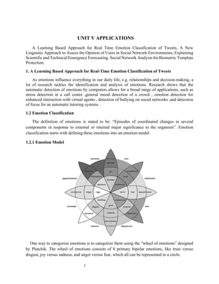
1.2.1 Emotion Model
One way to categorize emotions is to categorize them using the “wheel of emotions” designed
by Plutchik. The wheel of emotions consists of 8 primary bipolar emotions, like trust versus
disgust, joy versus sadness, and anger versus fear, which all can be represented in a circle.

2. 2
1.3 Architecture for Emotion Recognition for Real-Time Emotion Recognition
The Twitter client provides tweet data to the platform. This data is processed by the server and
the resulting classified emotion is sent back to the client. The architecture is designed based on the
principles of service-oriented architectures, wherein all components are implemented as REST
services. Important to notice is that no processing is done on the client itself, assuring that for
example smartphones are able to use emotion recognition, independent of their processing power
or storage capabilities. By using the generic concepts of service-oriented computing, the
architecture is also not restricted to emotion recognition in tweets. Due to its generic and scalable
design, it can be extended to detect emotions in different sorts of data, using other sensors as well,
or it can even be extended to provide multi-modal emotion recognition where the precision of the
classification of emotions is improved by combining different media
1.4 Emotion Recognition on Twitter
Twitter was founded in 2006 and its popularity keeps rising every day. Tweeting can be done
from various platforms, ranging from websites, mobile apps to even toasters.1 As it is possible to
tweet from a broad range of devices, Twitter is a good medium to gather data for text classification.
1.4.1 Dataset
The dataset used is part of the large dataset from Wang et al. Wang et al. initially started of
with 5 million tweets, which were slimmed down to 2.5 million tweets by using three filtering
heuristics. These filtering heuristics were developed on the 400 randomly sampled tweets. The
filters are as follows:
i. only tweets with hashtags at the end were kept, since those are more likely to correspond to
the writer’s emotion

3. 3
ii. tweets with less than 5 words were discarded
iii. tweets with URLs or quotations were also removed from the dataset.
The first step in order to be able to classify tweets is to preprocess them and standardize the text.
1.4.2 Preprocessing
First, the emotion hashtags are removed from the dataset in order to construct the ground-
truth data. If the hashtags are kept in the dataset, data leakage [20] would be created which results
in an unrealistically good classifier. The usernames which are lead by the at sign are kept in the
dataset. The next step consist of stemming, which reduces words to their stem.The second step in
classifying the short Twitter messages is to convert them to a feature space which can be used as
input for various machine learning algorithms. As it is important to choose both good and
sufficient features, the next section discusses the chosen feature extraction methods in more detail.
1. 4.3 Feature Extraction Methods
The feature extraction methods transform words and sentences into a numerical representation
(feature vectors) which can be used by the classification algorithms. In this research, the
combination of N-grams and TF-IDF feature extraction methods is chosen in order to preserve
syntactic patterns in text and solve class imbalance respectively.
1.4.3.1 N-Gram Features
In the field of computational linguistics and probability, an N-gram is a contiguous sequence
of N items from a given sequence of text or speech. An N-gram of size 1 is referred to as a
“unigram”, size 2 is a “bigram”, size 3 is a “trigram”. An N-gram can be any combination of
letters, syllables, words or base pairs according to the application. The N-grams typically are
collected from a text or speech corpus. N-grams are used to represent a sequence of N words,
including emoticons, in the training set and used as features to convert the tweets to the feature
space. Table 2 shows an example for converting a tweet into the feature space using unigrams,

4. 4
bigrams and trigrams. As can be seen in Table 2, there are 27 possible features for the given
example. In this research a combination of 1, 2 and 3 g is used which are then passed to the TF-
IDF algorithm.
5.3.2 Term Frequency-Inverse Document Frequency (TF-IDF)
As can be seen in Table 1, the dataset suffers a major imbalance, for example there are
significantly less tweets belonging to the class “fear” and “surprise” than to the other classes. In
order to see if this imbalance also reflects in the classification results when using occurrence to
construct the feature vectors, a test is done. In this test the tweets are transformed to feature vectors
by using the bag of word representation together with word occurrence. When these feature
vectors are constructed, they are used by a stochastic gradient decent (SGD) classifier with
modified huber loss . When looking at the results presented in Table 3, it is safe to state that the
imbalance can be detected.
To avoid these potential discrepancies, the number of occurrences of each word in a document
is divided by the total number of words in the document, called normalization. These new features
are called Term Frequencies (TF). Additionally, weights for words that occur in many documents
can be downscaled making them less dominant than those that occur only in a small portion of the
corpus. The combination of term frequencies and downscaling weights of dominant words is
called Term Frequency Times Inverse Document Frequency (TF-IDF).

5. 5
By composing the vocabulary for the feature vectors based on the dataset, the feature vectors
will be very high dimensional. But by combining TF-IDF and the N-grams method, a feature
vector will be very sparse. This can be beneficial if the used algorithms can work with sparse data.
2. A New Linguistic Approach to Assess the Opinion of Users in Social Network
Environments
Opinion mining is often viewed as a sub-field of sentiment analysis that, as the discourse
analysis or the linguistic psychology, seek to evaluate affective state through the analyze of natural
language. Nevertheless, many researchers define sentiment, loosely, as a negative or a positive
opinion.
2.1 Methodology
The core of our proposal consists in to take advantage of this natural relation in order to build
a contextualized lexicon that will be used to compute the opinion of an unknown text. In order to
validate our approach, we propose two experiments allowing to compare two methods of lexicons
generation. The first one uses the polarity-length relation. The second uses the seeds method. Both
experiments use the same set of data.
2.2 Experimental Validation of the Polarity-Length Method
In order to have a synthesis of the performances, we define 3 classes of opinions with their
rating (negative: 1–2 stars, neutral: 3, positive: 4–5 stars). The estimated opinion was computed
from the textual comment in order to fit the same scale (i.e. adapted from the Pij formula). In the
ideal situation the user stars rating should correspond to the computed one. The sensitivity of the
L size on the performances was evaluated with 8 tested sizes (from 364 to 7053 kB). The
performances are reported in the two following tables. The Table 2 presents the ratios with the
final consensus lexicons. These results of the full automated process can be compared with that of
the Table 3 with the best values during the 20 steps. This comparison shows that most of the time
the consensus lexicons give the best results. We can see that the size of the learning set is not a
clear criterion to have good performances (see in Table 2, F-index for 5014, 6124 and 7053 kB).

6. 6
Inorder to have a general view of the performances, we computed the average result with 4 learning
sets (average of 7172 reviews) an 4 validation sets (average 716 reviews). We applied the main
algorithm Polarity-length lexicon processing to each learning set and we measured the results on
each validation set. The statistical data corresponding to these 16 tests are reported in the Table
5.of view. Before this point of equilibrium,the content of the lexicons is still too random to allow
to identify the appropriate polarity.

7. 7
2.3 Seeds Based Method
The use of seeds seems to be the most powerful actual method but the choice of the initial key
words (the seeds) may have a strong influence on the final results. In this part of the experiment,
we take again the learning set that provide the better results (7053 kB) and the validation set and
we build the final lexicon on the basis of the seeds method. In order to show the sensitivity to the
initial seeds, we use four examples of 6 seeds (3 positives and 3 negatives) and we compute the
precision, recall and F ratio. The first set provides equivalent performance compared with our
method. In the second and the third set we changed only one world respectively with negative (set
2) and positive polarity (set 3). In the last set, we change several words for each polarity.
1. Seeds set 1: super, excellent, perfectly, bad, poor, expensive;
2. Seeds set 2: super, excellent, perfectly, bad, noisy, expensive;
3. Seeds set 3: super, excellent, recommend, bad, poor, expensive
4. Seeds set 4: good, excellent, friendly, poor, noise, bad;
The results show clearly that the seeds method is very sensitive to the choice of the worlds
even with a careful attention to the context (here, users’ comments on hotels). The case of the last
set is very interesting. We can observe that even with words that are evidently consistent in polarity
and in context, the performances are very bad. The reason is probably due to the representativity

8. 8
level of the seeds words in the learning set. It is important to say that each of these words is present
in the learning set but with a different frequency of occurrence (Table 6).
2.4 Comparison Between Methods
The most of the studies obtain more than 80% of accuracy. Moreover, we see that the seeds
and polaritylength method have at best, similar performances but with less stable results for seeds
method that in addition is more knowledge greedy. It needs more prior knowledge and the process
has to be controlled precisely (lexicon generation). Indeed, the seeds method needs either a
linguistic and a domain expertise in order to chose the most accurate seeds words or a good
learning set in order to statistically compensate the lack of representativity of a specific seed. The
lesser stability of this method could be explained by the difficulty to evaluate the added value of
this expertise and the effort necessary to gather the proper learning context.
3. Explaining Scientific and Technical Emergence Forecasting
In decision support systems such as those designed to predict scientific and technical
emergence based on analysis of collections of data the presentation of provenance lineage records
in the form of a human-readable explanation has been shown to be an effective strategy for
assisting users in the interpretation of results.
3.1 Background on the ARBITER System
ARBITER addresses emergence forecasting in a quantifiable manner through analysis of full-
text and metadata from journal article and patent collections.
We break ARBITER into four parts: (i) a highlevel overview of ARBITER’s infrastructure,
(ii) how prominence forecasts are managed through probabilistic reasoning, (iii) how evidence and
hypotheses are formally expressed through ontological modeling, and (iv) how ARBITER records
reasoning traces as lineage records to link hypotheses back to evidence.

9. 9
3.2.1ARBITER’s System Infrastructure
ARBITER’s system architecture provides a high-level overview of ARBITER’s processing
routines, carried out in the following sequence: First, documents are analyzed to obtain feature
data, consisting of statistics such as the total number of funding agencies referenced by publication
year. Second, feature data is recorded to the RDF knowledge base. Third, feature data is read by a
second set of analysis routines to calculate emergence-oriented indicators. Fourth, indicators are
recorded back to the RDF knowledge base. Fifth, provenance records that track the indicator
derivations are made accessible to the explanation system for analysis.
Once a set of indicators and feature data has been established from the document corpora,
ARBITER may then check the prominence of a term/publication person represented within the
corpora, based on a supplied query. ARBITER utilizes Bayesian probabilistic models, to establish
prominence scorings through observed indicator values. In turn, to express hypotheses of
prominence, evidence for prominence (indicators, features), as well as formal relationships
between hypotheses and evidence, an RDF/OWL based encoding strategy is used.
3.2.2Encodings for Evidence and Hypotheses
Content structuring for ARBITER’s RDF knowledge base is established using an OWL-
based ontology. This ontology serves three purposes: First, to represent hypotheses of prominence.
Second, to express traces of reasoning steps applied to establish hypotheses discussed in greater
detail. And third, to formally express evidence records based on data identified in publication
collections. Combined, these three forms of content are used as input to ARBITER’s explanation
component.

10. 10
Each evidence instance corresponds to a unique Indicator and has a generic degree of relevance
to the hypothesis as well as a more specific weight in supporting, or disconfirming, the specific
hypothesis. In turn, each indicator has a value and is associated with both a generic mode of
computation as well as a more detailed computation based on feature values.
Therefore, ARIBTER’s ontology imports the Mapekus Publication ontology for describing
documents and adds representations for document features, indicators, indicator patterns, and high
level network characteristics.

11. 11
3.2.3 Probabilistic Modeling
One approach to overcoming the opaqueness of probability calculations is to impose some
structure on the probability model. Bayesian networks are a step in this direction since they encode
meaningful relations of dependence or independence between variables. Bayesian networks are
directed graphs in which the nodes represent random variables and the links capture probabilistic
relations among variables. Nodes in Bayesian networks are typically categorized as observable or
unobservable.
Let PROM be the prominence variable that is the root of a given Naive Bayes net model and
let IND1, IND2,…,INDn be the indicator variables for PROM. A Naive Bayes net specifies the
conditional probability distribution p(INDi|PROM) for each indicator variable INDi. The structure
of a Naive Bayes net implies that the child variables are probabilistically independent of one
another conditional on the root variable. This implies that we can compute the posterior probability
of the prominence variable given values for the indicator variables by the formula:
The Naive Bayes nets serve as baselines giving competitive performance on the prediction
problems of interest in ARBITER. In more recent work, we have implemented Tree Augmented

12. 12
Naive Bayes models, which remove the assumption of conditional independence among the
indicator variables.
3.2.4 Trace Generation
A record of this reasoning consists of a description of what evidence was entered, which nodes
in the Bayes net the entered evidence immediately affected, and what the weight of evidence is for
each piece of evidence entered. When a piece of evidence is entered into the Bayes net, in the form
of an assignment of a value to an indicator variable, a record is made of the propagation of that
evidence through the net. We record the value assigned to the indicator node, the change in the
probabilities for the parent pattern variable, and the consequent effect on the probabilities for the
hypothesis variable. This information is used to generate a trace of the reasoning in RDF, expressed
using the vocabulary ARBITER’s explanation ontology.
3.3 Explaining Prominence Forecasting
Science and technology analysis systems such as ARBITER have been successfully used to
make predictions about constrained information spaces based on available evidence.Our
infrastructure design has been driven by two goals: utilize lineage records to support transparency
into emergence forecasting by exposing both indicator values and probabilistic reasoning steps
applied, and develop strategies for providing context-aware drilldowns into evidence underlying
presented indicators.
3.3.1 Trace-Based Explanation
1. Reference Period: Denotes the most recent year in which documents from ARBITER’s
corpus are considered.
2. Forecast Period: The year the prominence prediction is made for.

13. 13
3. Predicted Prominence: A scoring of the prominence for a given patent, term or
organization.
4. Evidence Table: A table of all indicators considered by ARBITER in making the
prominence prediction.
5. Evidence: This column of the evidence table lists names of indicators considered.
6. Value: This column lists indicator values calculated.
7.Weight of Evidence: Weight of evidence is based on the amount the probability of the
conclusion increased or decreased upon finding out the value of a given indicator. Positive weights
of evidence indicate that the evidence raises our prior expectation of prominence while negative
values indicate that the evidence lowers our expectation of prominence.
8. Evidence Entry: These correspond to individual indicators applied as evidence.
The items listed correspond to dynamic content generated by ARBITER during runtime.
3.3.2Drilling Down into Indicator Evidence

14. 14
Two drilldown strategies—both incorporating information supplementing lineage records—
were considered for presenting evidence records: In the first, the data used to calculate individual
evidence values was exposed through evidence-specific visualization strategies; in the second,
evidence values and supporting data across information spaces were compared. Figure 6 provides
an example drilldown visualization for an indicator tracking growth in the number of organizations
represented in a document corpus. Here, our system is able to determine an appropriate
visualization strategy, using a bar chart based on the OWL class of the indicator present in
ARBITER’s ontology. The data used to generate the bar chart is retrieved from ARBITER’s
dynamically generated knowledge base at runtime.
In addition to providing visualization strategies, ARBITER’s ontology provides written
statements about indicators, such as general descriptions and their rationale for usage. This
information can be retrieved on-demand from an indicator’s drilldown page.
4. Social Network Analysis for Biometric Template Protection
Social network based feature analysis confirms the domain transformation. It is
computationally very hard to regenerate the original features from the social network matric value.
This domain transformation confirms the cancelability in biometric template generation. To ensure
the multi-level cancelability random projection is used to project social network based feature.

15. 15
4.1 Methodology
In the first stage of the transformation is the 2-Fold random cross folding. The outcome of
the process is two sets of a feature that are cancelable. Random indexes are used to generate two
folds. Distance based features are calculated from Fold 1 and Fold 2. Distance features are then
projected using random projection that transforms the original m-dimensional data to n-
dimensional.
4.1.1 2-Fold Random Cross Folding
In this step of the proposed system, biometric raw data are randomly split into n blocks. These
blocks are then processed. Figure 3 shows the general block diagram for random splitting. Raw
face or ear biometric features are divided into two equal parts.A pseudorandom number generation
algorithm is used to split the raw features into two parts. In the Fig. 3, we have presented the
method of random selection. From NxN face template, m random features are selected and named
as Fold 1.Other m features are Fold 2, where m=NxN/2.

16. 16
Instead of selecting local features of face like lips, eye etc., we have selected random features.
Randomness of the features ensures some properties of cancelability.An example of 2-Fold Cross-
Folding is shown in Fig. 3. This example takes 8 × 8 blocks of pixels. The partition of the block is
based on the random indexes. Each cell of the block represents a pixel.
4.2 Feature Extraction Using Fisherface
From the idea of R. A. Fisher, Belhumeur et al., 1997 inspired to establish Fisherface (FLDA)
method for face recognition in different illumination condition where Eigenface method can fail.
They have designed a class specific linear projection method for face recognition to maximize the
interclass variation and minimize the intra class similarity.
Eigenface method finds total variation of data regardless of the class specification.Using
Fisherface method allows us to identify the discriminative class specific feature extraction.
Because of the class specification and discriminability of feature extraction, we have used
Fisherface method instead of Eigenface as a tool to find the features from cross-folded cancelable
biometric data.
4.3 Social Network Analysis

17. 17
Performance of the biometric feature depends on constructed network. Therefore, construction
of social network from the feature is very important task. Mechanism for virtual social network
construction should keep the discriminability of the features. Social Network is constructed from
the Fold 1 and Fold 2 features. In the first step correlation among the features are computed.
Correlation coefficients are taken because it is the relation between the two features sets. A
threshold is applied on the coefficients to find the social network. Correlation coefficients are
computed for all features, and it gives an adjacency matrix of relation. L1 or L2 distances are not
taken because of the feature extensive information loss. Using correlation instead can keep the
spatial relation among the feature, which can be the shape of the human face or ear. We have taken
two different networks from the adjacency matrix. It can be done by using upper and lower
triangulation.

18. 18
We named two networks as Social Network-1 and Social Network-2 . A weight is calculated
from features of Fold 1 and Fold 2. Distance based features are used to generate weights.
Eigenvalue centrality is measured for both networks. The cross products of both features are taken
to fuse them together. Figure 4 is the block diagram of the proposed social network based
cancelable fusion..
This process is cancelable because it satisfies the property of cancelable features. First, it is
computationally hard to reconstruct the original feature from the calculated features. Second, once
the cross fold indexes are changed, therefore, the feature relations as well as the constructed
network changed. Finally, features from social network are non-invertible which increases the
template security.
4.4 Validation of Virtual Social Network
Validation of the constructed social network can be done based on several values such as
betweenness centrality, clustering coefficient, degree centrality, eigenvector centrality etc. From
the analysis of the metric values we found that different metric gives better distribution of values
for different threshold values. We found the best betweenness for 65% of correlation values. For
clustering coefficient, degree centrality and eigenvector centrality 60% of the correlation values
gives the best distribution of social network metric values.
In the following sections, we have presented the computation for each of the centrality
measures. In 1972, Bonacich suggested that the eigenvector could be a good network centrality
measure. It can be computed form the largest eigenvalue of an adjacency.matrix. It assigns relative
scores to all nodes in the network. Assigning the score depends on the high-scoring and low-
scoring nodes [34].
For a social network G (V, E), if |V| is the number of vertices and A is the adjacency matrix
the eigenvector centrality of node v can be computed using Eqs. (1) and (2).
where M (v) is a set of neighbor node v and is constant can be computed form Eq. (2).

19. 19
In eigenvector centrality measure, eigenvector for highest eigenvalues are taken. Figure 7
shows the eigenvector centrality distribution for different correlation coefficient threshold.
Network construction using 60% of the correlation coefficient gives better convergence for the
centrality of the node (person). Uniqueness of the centrality measure is an important to provide
feedback to the classifier.

20. 20
4.5 Random Projection and Classification
The k-nearest neighbor (k-NN) is one of the simplest and powerful classifier for pattern
recognition. k-NN uses topological similarity in the feature space for object recognition [41]. It
uses a majority vote of the neighbors to establish the out-put. k is a small positive integer. If k =
1, it uses similarity distance between two objects. It is better to use odd numbers of k to address
the voting tie. There is different distance functions used in k-NN classifier. The similarity value of
k-NN algorithm can be calculated using Euclidean distance, cosine distance, city block distance
etc. [41]. In k-NN classifier, value of k is very important. For all types of system, optimization of
k is an important factor. Finding k can be brute force search or k means clustering. In brute force
search, systems are modeled for different values of k. The model that gives the best performance
is selected for k. Another way of optimization of k is using k means clustering. If a cluster is
optimal, it is possible to get best k from the distribution of classes in a cluster. After understanding
the feature characteristics optimal k is selected.