This project aims at simulating lid driven cavity flow problem using package MATLAB. Steady Incompressible Navier-Stokes equation with continuity equation will be studied at various Reynolds number. The main aim is to obtain the velocity field in steady state using the finite difference formulation on momentum equations and continuity equation. Reynold number is the pertinent parameter of the present study. Taylor’s series expansion has been used to convert the governing equations in the algebraic form using finite difference schemes.

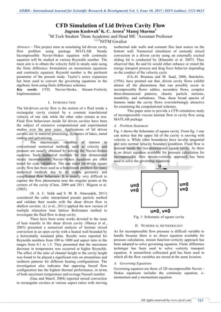
1. IJSRD - International Journal for Scientific Research & Development| Vol. 3, Issue 10, 2015 | ISSN (online): 2321-0613
All rights reserved by www.ijsrd.com 727
CFD Simulation of Lid Driven Cavity Flow
Jagram Kushwah1
K. C. Arora2
Manoj Sharma3
1
M.Tech Student 2
Dean Academic and Head ME 3
Assistant Professor
1,2,3
NITM Gwalior
Abstract— This project aims at simulating lid driven cavity
flow problem using package MATLAB. Steady
Incompressible Navier-Stokes equation with continuity
equation will be studied at various Reynolds number. The
main aim is to obtain the velocity field in steady state using
the finite difference formulation on momentum equations
and continuity equation. Reynold number is the pertinent
parameter of the present study. Taylor’s series expansion
has been used to convert the governing equations in the
algebraic form using finite difference schemes.
Key words: CFD, Navier-Stroke, Stream-Vorticity
Implementation
I. INTRODUCTION
The lid-driven cavity flow is the motion of a fluid inside a
rectangular cavity created by a constant translational
velocity of one side while the other sides remain at rest.
Fluid flow behaviours inside lid driven cavities have been
the subject of extensive computational and experimental
studies over the past years. Applications of lid driven
cavities are in material processing, dynamics of lakes, metal
casting and galvanizing.
The macroscopic variables of interest in
conventional numerical methods, such as velocity and
pressure are usually obtained by solving the Navier-Stokes
equation. Such numerical methods for two dimensional
steady incompressible Navier-Stokes equations are often
tested for code validation. The one sided lid-driven square
cavity flow has been used as a benchmark problem for many
numerical methods due to its simple geometry and
complicated flow behaviors. It is usually very difficult to
capture the flow phenomena near the singular points at the
corners of the cavity (Chen, 2009 and 2011. Migeon et al.
(2003)
(N. A. C. Sidik and S. M. R. Attarzadeh, 2011)
considered the cubic interpolated pseudo particle method
and validate their results with the shear driven flow in
shallow cavities. (Li et al., 2011) applied the new version of
multiple relaxation time lattices Boltzmann method to
investigate the fluid flow in deep cavity.
There have been some works devoted to the issue
of heat transfer in the shear driven cavity. (Manca et al.,
2003) presented a numerical analysis of laminar mixed
convection in an open cavity with a heated wall bounded by
a horizontally insulated plate. Results were reported for
Reynolds numbers from 100 to 1000 and aspect ratio in the
ranges from 0.1 to 1.5. They presented that the maximum
decrease in temperature was occurred at higher Reynolds.
The effect of the ratio of channel height to the cavity height
was found to be played a significant role on streamlines and
isotherm patterns for different heating configurations. The
investigation also indicates that opposing forced flow
configuration has the highest thermal performance, in terms
of both maximum temperature and average Nusselt number.
(Gau and Sharif, 2004) reported mixed convection
in rectangular cavities at various aspect ratios with moving
isothermal side walls and constant flux heat source on the
bottom wall. Numerical simulation of unsteady mixed
convection in a driven cavity using an externally excited
sliding lid is conducted by (Khanafer et al. 2007). They
observed that, Re and Gr would either enhance or retard the
energy transport process and drag force behavior depending
on the conduct of the velocity cycle.
(Ch.-H. Bruneau and M. Saad, 2006, Batchelor,
(1956), have pointed out that, driven cavity flows exhibit
almost all the phenomena that can possibly occur in
incompressible flows: eddies, secondary flows, complex
three-dimensional patterns, chaotic particle motions,
instability, and turbulence. Thus, these broad spectra of
features make the cavity flows overwhelmingly attractive
for examining the computational schemes.
This paper aims to provide a CFD simulation study
of incompressible viscous laminar flow in cavity flow using
MATLAB package
A. Problem Statement
Fig. 1 shows the Schematic of square cavity. From fig. 1 one
can notice that the upper lid of the cavity is moving with
velocity u. While other boundaries have no-slip tangential
and zero normal velocity boundary condition. Fluid flow is
laminar inside the two-dimensional square cavity. As there
is no direct equation available for pressure calculation for
incompressible flow stream-vorticity approach has been
used to solve the governing equations
Fig. 1: Schematic of square cavity
II. NUMERICAL METHODOLOGY
As for incompressible flow pressure is difficult variable to
handle because there is no direct equation available for
pressure calculation, stream function-vorticity approach has
been adopted to solve governing equation. Finite difference
technique has been used to solve vorticity transport
equation. A nonuniform collocated grid has been used in
which all the flow variables are stored at the same location.
A. Governing Equations
Governing equation are those of 2D incompressible Navier -
Stokes equations includes the continuity equation, x-
momentum and y-momentum equation

2. CFD Simulation of Lid Driven Cavity Flow
(IJSRD/Vol. 3/Issue 10/2015/156)
All rights reserved by www.ijsrd.com 728
B. Continuity Equation
C. Momentum Equations
1) X-Momentum Equation
( )
2) Y-Momentum Equation
( )
D. Stream-Vorticity Implementation
As governing equation involves the pressure term and there
is no direct equation for calculating pressure it is difficult to
calculate pressure in the incompressible flow. Stream-
vorticity implementation will eliminate the pressure term
from governing equation by cross-differentiation of the x-
momentum and y-momentum equation and makes the
problem easy to construct numerical schemes.
1) Velocity And Stream-Function Relationship
2) Vorticity And Stream-Function Relationship
( )
E. Vorticity Transport Equation
( )
The above equations can be non-dimensionalized by non-
dimensional parameters listed below
⁄
F. Vorticity and Stream-Function Relationship
( )
G. Vorticity Transport equation
( )
H. Taylor’s Series Expansion
The difference approximation can be done using Taylor-
series expansion or Taylor’s formula. Taylor-series
expansion for T(x+∆x, y) about (x, y) can be represented as
( ) ( )
( ) ( ) ( )
( )
From equation 4.1 we can find the algebraic form
of first order partial differential term for forward scheme by
rearranging the term as,
( ) ( ) ( ) ( )
Changing to i, j notation, we can write the above equation
as,
Where truncation error (T.E.) is the difference between the
partial derivative and its finite-difference representation. We
can also write the above eq. as,
( )
Where O(∆x) represents the order of term ∆x and
higher, which has been neglected during finding the
approximation.
Similarly,
( )
( )
( )
( )
III. GRID GENERATION
Physical domain has been discretized into small rectangular
four nodded elements. A non-uniform collocated grid has
been used for better accuracy at the walls of the enclosure.
A collocated grid is what in which all the field variables
(vectors as well as scalars) are defined at the same point of a
cell. Figure 2 shows the non-uniform collocated grid where
element φ (i, j) represents the velocity component, stream-
function, vorticity and temperature at the ith and jth node.
Fig. 2: Schematic diagrams of computational domain and
grid layout
IV. RESULTS
Figure 3 and 4 represents the contours of stream lines,
vertical velocity and horizontal velocity for different grid
size, stream lines actually represents the flow of the fluid
inside the cavity. From the contours one can notice that
difference between the stream lines near the upper lid is
very small which means that flow of the fluid is very high
which actually represents the lid-driven upper wall.

3. CFD Simulation of Lid Driven Cavity Flow
(IJSRD/Vol. 3/Issue 10/2015/156)
All rights reserved by www.ijsrd.com 729
Fig. 3: Contour plot of stream function for characteristics
Fig. 4: Contour plot of vertical and horizontal velocities for
characteristics
V. CONCLUSION
 Taylor series helps in converting the partial equations
into algebric form.
 Software like MATLAB can be used to simulate the
Navier-stokes equation.
 Contours of strem function and velocities have been
presented.
 Increment in grid size affects the solution of the
problem.
 From the contours one can notice that difference
between the stream lines near the upper lid is very
small.
 Flow of the fluid is very high which actually represents
the lid-driven upper wall.
REFERENCES
[1] Chen S, A large-eddy-based lattice Boltzmann model
for turbulent flow simulation. App. Mathe. & Comp.,
215, pp. 591–595.
[2] N. A. C. Sidik and S. M. R. Attarzadeh, An accurate
numerical prediction of solid particle fluid flow in a lid-
driven cavity. Intl. J. Mech., 5(3), pp. 123-128.
[3] S.L. Li, Y.C. Chen, and C.A. Lin. Multi relaxation time
lattice Boltzmann simulations of deep lid driven cavity
flows at different aspect ratios. Comput. & Fluids,
45(1), pp. 233-240.
[4] A.J. Chamkha, Hydromagnetic combined convection
flow in a vertical lid-driven cavity with internal heat
generation or absorption, Numer. Heat Transfer, Part A,
vol. 41, pp. 529-546.
[5] K.M. Khanafer, A.M. Al-Amiri and I. Pop, Numerical
simulation of unsteady mixed convection in a driven
cavity using an externally excited sliding lid, European
J. Mechanics B/Fluids, vol. 26, pp.669-687.
[6] G.K. Batchelor. On Steady Laminar Flow with Closed
Streamlines at Large Reynolds Numbers. J. Fluid
Mech., 1, pp. 177–190.