In this paper, a problem of allocation and sizing of multiple active power-line conditioners (aplcs) in power systems is handled with novel formulation. The utilized objective function comprises two main factors such as reduction of total harmonic distortion and the total cost of active power-line conditioners (aplcs). The formulated problem is solved by optimization technique SHUFFLE FROG LEAP ALGORITHM (SHFLA) using MATLAB. To evaluate the competence of the proposed formulation, the IEEE 18-busdistorted distribution test system is employed and investigated with various number of aplcs placement. These cases are based on the discrete and limited size for aplcs, requiring the optimization method to solve the constrained and discrete nonlinear problems. The comparison of results in this paper showed that the proposed SHFLA is the most effective result among others in determining optimum location and size of APLC in distribution systems.

1. Indonesian Journal of Electrical Engineering and Computer Science
Vol. 5, No. 2, February 2017, pp. 267 ~ 276
DOI: 10.11591/ijeecs.v5.i2.pp267-276  267
Received September 12, 2016; Revised December 20, 2016; Accepted January 1, 2017
Optimal Placement and Sizing of Active Power Line
Conditioners for Minimizing Power Quality Problems
Swathisriranjani M*
1
, Mohananthini N
2
, Ranjitha M
3
, Baskar S
4
, Kavitha D
5
1, 2, 3, 4
Muthayammal Engineering College, India
5
Thiagarajar College of Engineering, India
*Corresponding author, e-mail: mail2swathieee@gmail.com
Abstract
In this paper, a problem of allocation and sizing of multiple active power-line conditioners
(aplcs) in power systems is handled with novel formulation. The utilized objective function comprises two
main factors such as reduction of total harmonic distortion and the total cost of active power-line
conditioners (aplcs). The formulated problem is solved by optimization technique SHUFFLE FROG LEAP
ALGORITHM (SHFLA) using MATLAB. To evaluate the competence of the proposed formulation, the
IEEE 18-busdistorted distribution test system is employed and investigated with various number of aplcs
placement. These cases are based on the discrete and limited size for aplcs, requiring the optimization
method to solve the constrained and discrete nonlinear problems. The comparison of results in this
paper showed that the proposed SHFLA is the most effective result among others in determining
optimum location and size of APLC in distribution systems.
Keywords: active power-line conditioner (APLC), harmonics, shuffle frog leap algorithm (SHFLA),
optimal allocation and sizing of APLCs (OASA) problem
Copyright © 2017 Institute of Advanced Engineering and Science. All rights reserved.
1. Introduction
The APLC is converter based compensation device and it is designed to improve
the power quality of the entire distribution system by injecting corrective harmonic current at
selective (sensitive) buses. APLC consists of set of shunt active filters. APLC’s placement,
sizing and compensation levels (e.g., orders, magnitudes and phases of injected current
harmonics) are optimally placed to improve the power quality of the entire distribution system.
The number of required APLC units depends on the distortion level, the nature of the
distribution system and the type of nonlinear loads as well as the quality of electric power.
Although passive filters are widely employed due to their simplicity and economical
cost, active power line conditioner is deemed the most efficient device for the reduction of
harmonic level. The advantages of active power line conditioners are well established in
literatures. Despite of the advantages, installation of active power line conditioners in a power
distribution system is a very complicated problem. The harmonic standard, locations and sizes
of APLCS, as well as the injection currents spectra of APLCs must be thoroughly considered.
In addition, the sizes of the commercially available APLCs have discrete values. Despite a
large number of benefits provided by APLCs, their huge installation and operation costs
prevent electrical engineers from employing these profitable instruments without any
restriction at all buses in power distribution systems.
Hence, in a large distribution system, it becomes necessary to locate suitable places
for APLC installation to reduce these distortions and fixing their sizes is also essential. Owing
to this fact, a variety of solution techniques have been utilized to solve the APLCs allocation
and sizing problem. These techniques are mainly categorized into two groups:
1) Allocation of only one APLC and
2) Allocation of multiple APLCs.
The authors Grady & Samotyj (1992) and Chang & Grady (1994) have introduced the
initial steps toward solving Optimal Allocation and Sizing of APLCs (OASA) problem.
Zhao, et al., (2001) have proposed chance constrained programming for optimal
planning of harmonic filter in distribution systems. Chang, et al., (2001) have proposed a

2.  ISSN: 2502-4752
IJEECS Vol. 5, No. 2, February 2017 : 267 – 276
268
combined differential evolution/multiple gradient summation approach for reducing harmonic
distortion using APLCs. The goal of this approach is to minimize the total injection currents of
APLCs, while satisfying standard constraints such as the individual harmonic voltage
distortion, total harmonic voltage distortion (THD) limits, and the commericially available
discrete sizes of the APLCS. Iman Ziari, et al., (2010) have presented a PSO algorithm for
allocation and sizing of multiple Active Power Line Conditioners (APLCs) in power systems.
They considered the objectives of minimizing the APLC rating as well as THD.
In these works, the cost of APLC is not considered. The realistic investment cost of an
APLC is divided into two different parts, constant cost and the incremental cost. The constant
cost, which is not related to the APLC rating called fixed installation cost, ie constant and The
incremental cost is proportional with the APLC rating. If APLC rating is the objective to be
minimized, it indirectly results in ignoring the fixed installation cost. This assumption
influences the results and leads the optimization method in use of a number of APLCs with
higher investment cost.
Also, In all these works, the standard IEEE 18 bus distorted distribution system is
taken for the case study and in this system, the non linear loads occurs at only at three to five
buses. Hence the problem convergence is fast and the allocation of APLC units falls within
these buses. Luis Sainz, et al., (2012) have explained the increase of nonlinear loads (NLLs)
in supply networks that has led to an increase of harmonic content in supply currents. Thus
in practical, the sizes of non linear loads are increasing greatly and cannot be restricted to
limited number of buses. Hence in this work, it is considered about 11 buses are having non
linear loads and the APLC placement may be in any of the 18 buses.
Iman Ziari, et al., (2012) have considered the problem with the objective of cost
minimization of APLCs. The fixed cost of an APLC is taken as 90000$ and the incremental
cost of an APLC is taken as 720000$ per 1 pu (Zhao 2001).Using these values, the realistic
investment cost of APLC is calculated. The objective function is the investment cost of APLCs
and the constraints are voltage THD and the individual voltage harmonic distortion which
should be maintained less than 5% and 3%, respectively. Hence in this work, APLCs
placement and sizing are evaluated for a distorted distribution system considering two main
objectives such as reduction in THD as well as APLC cost under the presence of more
number of non linear load buses.
2. Problem Formulation
The APLC is modeled as a set of current sources which inject different order of
harmonics to the point of common coupling. To assume amplitude and phase angle for an
APLC current, the phasor model is shown by:
= + (1)
Where,
APLC current at bus for harmonic order ;
real part of APLC current at bus for harmonic order ;
imaginary part of APLC current at bus for harmonic order ;
The indices and represent the real and imaginary parts of the APLC current,
respectively.
The objective is to minimize the total investment cost of APLCs and the total harmonic
distortion that occur in the system. The constraints are individual harmonic distortion. THD is
also introduced as one of the constraints. The investment cost of an APLC includes of the
constant cost and the incremental cost. The constant cost, called fixed installation cost, is
constant and is not related to the APLC rating, e.g. the required cost for securing and
purchasing land. The incremental cost, e.g. the purchase cost, is proportional with the APLC
rating. The objective function is formulated as follows:
= + (2)

3. IJEECS ISSN: 2502-4752 
Optimal Placement and Sizing of Active Power Line Conditioners for… (Swathisriranjani M)
269
Where and are weight factors.
can be formulated as follows:
(3)
= (4)
Where: number of buses
- maximum considered harmonic order - voltage at bus for harmonic order
- THD at bus
can be formulated as follows:
(5)
Where: -constant cost of APLCs
- incremental cost of APLCs
- rating of an APLC located at bus m which is proportional with its current.
NB - number of APLC buses
= k (6)
- the set of harmonic orders.
- the set of bus installations of the APLCs.
(7)
- the base unit size of the APLC.
- maximum size of the APLC. The constraints are given as follows
i = 1, . . . ,M
h (8)
Where (8) is the individual harmonic voltage distortion for each bus within the limit, and
is usually 3%. Equation 7 denotes that the sizes of APLCs are discrete in nature.
- the harmonic voltage at bus i for harmonic h.
- the fundamental frequency voltage at bus i.
Due to the occurrence of parallel resonance, the most serious voltage harmonic
distortion may occur at those buses, where there is no nonlinear load but there is a capacitor
installed. A bus where exists no nonlinear load but a high level of voltage harmonic distortion
may not be the perfect candidate location to install APLCs to eliminate harmonics (Chang
2000). Also, the rating of APLC depends on the individual harmonic current injection into the
bus by APLC. Hence, there is a possibility that, wrong current injections may lead to
excessive rating of APLC as well as increase in THD levels. These are some of the reasons
that make the problem with many local solutions and so, search space is wider.
3. Shuffle Frog Leap Algorithm (SHFLA)
The SFLA is a optimization method that the memetic evolution of a group of frogs
when seeking for the location that has available of food. The algorithm consists of local search
and global information exchange. The SFL algorithm involves a population of possible

4.  ISSN: 2502-4752
IJEECS Vol. 5, No. 2, February 2017 : 267 – 276
270
solutions defined by a set of frogs (i.e. solutions) that is partitioned into subsets referred to as
memeplexes. The different memeplexes are considered as different cultures of frogs, each
performing a local search. Within each memeplex, the individual frogs hold ideas, that can be
influenced by the ideas of other frogs, and evolve through a process of memetic evolution.
After a number of memetic evolution steps, ideas are passed among memeplexes in a
shuffling process. The local search and the shuffling processes continue until convergence
criteria are satisfied Frog’s fitness can be simply defined as:
fitness=f(X)+C (9)
Where f(X) is the cost function to be optimized, and C is a constant chosen to
ensure that the fitness value is positive. Afterwards, the frogs are sorted in a
descending order according to their fitness. Then, the entire population is divided into m
memeplexes, each containing n frogs, in such a way that the first frog goes to the first
memeplex, the second frog goes to the second memeplex, the mth frog goes to the mth
memeplex, and the (m+1)th frog goes back to the first memeplex,
According to the original frog leaping rule, the position of the worst frog is updated as
follows:
D=r.(Xb-Xw) (10)
Xw (new) = Xw + D,( |D| <Dmax ) (11)
Where: r is a random number between 0 and 1;
Dmax is the maximum allowed change of frog’s position in one jump.
If this leaping produces a better solution, it replaces the worst frog. Otherwise, the
calculations in Equation (10) and (11) are repeated but respect to the global best frog (i.e. Xg
replaces Xb). If no improvement becomes possible in this case, the worst frog is deleted and
a new frog is randomly generated to replace it.The calculations continue for a predefined
number of memetic evolutionary steps within each memeplex, and then the whole population
is mixed together in the shuffling process. The local evolution and global shuffling continue
until convergence criteria are satisfied. Usually, the convergence criteria can be defined as
follows:
1. The relative change in the fitness of the best frog within a number of consecutive
shuffling iterations is less than a pre-specified tolerance;
2. The maximum user-specified number shuffling iterations is reached. The SFLA will
stop when one of the above criteria is arrived first.
4. Methodology
The solution methods aim at determining optimal allocation and sizing of APLC.The
problem solving involves load flow analysis, harmonic flow analysis and calculation of APLC
cost for each feasible solution. Hence, Fundamental and Harmonic load flow analysis are
integrated with the optimization technique, in order to obtain the fitness functions for the
individual harmonic distortion and total harmonic distortion that occur in the distribution
system. Load-Flow studies are performed to determine the steady- state operation of an
electric power system.
4.1. Load Flow Analysis
A load-flow study calculates the voltage drop in each feeder, the voltage at each bus,
and the power flow in all branch and feeder circuits. The conventional methods for load flow
analysis include Single-Line Equivalent Method, Very Fast Decoupled Method, Ladder
Technique, Power Summation Method and Backward and Forward Sweeping Method. An
effective approach proposed by Alsaadi & Gholami (2009) for distribution power flow
solutions is utilized in this work. The special topological characteristics of distribution networks
have been fully utilized to make the direct solution. Two matrices namely the Bus-Injection to
Branch-Current matrix (BIBC) and the Branch-Current to Bus Voltage matrix (BCBV) and a
simple matrix multiplication are used to obtain power flow solutions.

5. IJEECS ISSN: 2502-4752 
Optimal Placement and Sizing of Active Power Line Conditioners for… (Swathisriranjani M)
271
For distribution networks, the equivalent current injection based model is more
practical. For bus i, the complex load ‘ ’ is expressed by:
Si=Pi + j Qi (12)
Where i = 1, 2, 3, ..., M
And the corresponding equivalent current injection at the kth iteration of solution is:
Ii
k= (Pi + j Qi )/ Vi
k* (13)
Where Vi
k and Ii
k are the bus voltages and equivalent current injection of bus i at k
th
iteration, respectively.
[B]=[BIBC]*[I] (14)
Where BIBC is a bus injection to branch current matrix and the BIBC matrix is a upper
triangular matrix which contains 0’s and 1’s only.
The relation between branch currents and bus voltages can be obtained by using the
following equation.
V(m2) = V(m1) – B*Z (15)
Where, m1, m2 are the sending and receiving ends.
4.1.1. Harmonic Load Flow Analysis
The conventional harmonic power flow method is used. The bus voltage for all
harmonic orders is then calculated by multiplying the injecting currents and the impedance
matrix is:
(16)
Where and are the bus voltages and the injecting current vectors for hth
harmonic order, respectively. is the admittance matrix for hth harmonic order and is
determined for all the harmonics orders considered.The admittance matrix is formed using
direct inspection method (Wadhwa 2010)
In this procedure, the current injecting to buses, , is obtained using the
following equation:
(17)
Where and the are injecting current vectors related to the nonlinear loads and
APLCs, respectively.
The APLC currents are modified using Equations (19) and (20) to convert it as a
discrete structure using integer optimizer.
= × (18)
(19)
Here ‘round’ will convert the float variable to the nearest integer. is a correction factor to
correct the rating of the APLC located at bus m as integer multiples of Base Unit Rating (Ib) of
APLCs. As mentioned, Ib is assumed to be 0.01p.u.

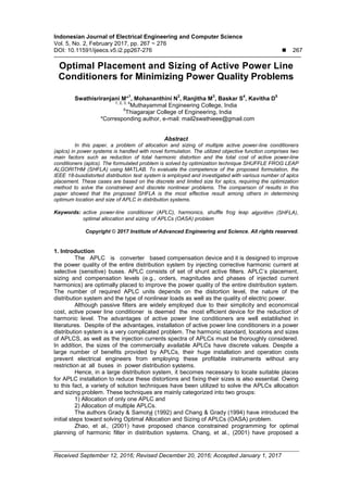
6.  ISSN: 2502-4752
IJEECS Vol. 5, No. 2, February 2017 : 267 – 276
272
4.2. Algorithmic Steps to Solve OASA Problem
The sequential steps are as follows:
Step 1: Create an initial population of P frogs generated randomly.
SFHLA Population =[X1,X2,…,Xp]p×n
Where, P=m×n,
N = number of APLC=3
m = number of memplexes= 5and
n = number of frogs in each memeplex=20.
Step 2: For each individual population, calculate fitness function. Fitness
function=THD+COST. THD and COST formula is given in the equation (4) & (5).
Sort the population increasingly and divide the frogs into m memplexes each holding n
frogs such that P=m×n. The division is done with the first frog going to the first memplex,
second one going to the second memplex, the mth frog to the mth memplex and the
m+lth frog back to the first memplex.
Step 3: Within each constructed memeplex, the frogs are infected by other frogs'
ideas; hence they experience a memetic evolution. Memetic evolution improves the quality of
the meme of an individual and enhances the individual frog’s performance towards a goal.
Below are details of memetic evolutions for each memeplex.
1. Set m1=0 where m1 counts the number of memeplexes and will be compared with
the total number of memeplexes m. Set y1=0 where y1 counts the number of evolutionary
steps and will be compared with the maximum number of steps (ymax), to be completed
within each memeplex.
2. Set m1=m1+1
3. Set y1=y1+1
4. For each memeplex, the frogs with the best fitness and worst fitness are identified
as Xw and Xb respectively. Also the frog with the global best fitness Xg is identified, and then
the position of the worst frog Xw for the memeplex is adjusted such as Equation (10)
and (11). If the evolutions produce a better frog (solution), it re-places the older frog,
otherwise Xb is replaced by Xg in (10) and the process is repeated. If no improvement
becomes possible in this case a random frog is generated which replaces the old frog.
5. If m1<m, return to step3-b.
If y1<ymax, return to step 3-c, otherwise go to step 2.
Step 4: Check the convergence. If the convergence criteria are satisfied stop,
otherwise consider the new population as the initial population and return to the step 2. The
best solution is that we get both THD (should be less than 5% within the standard limit) and
cost are to be minimum.
5. Results and Discussion
In this case, the modified IEEE 18- bus system (Iman Ziari & Alireza Jalilian 2012) is
used as a test system. The base voltage is 12.5kV and base power is 10MVA. In this
system, 16 buses (Bus number 1 to 16) are assumed as candidate for installation of APLCs.
The bus and line data are provided in reference [7]. The nonlinear loads are modeled
as identical harmonic current sources. In this system, eleven identical harmonic current
sources are employed as nonlinear loads and located at buses 3,4,5,6,7,8,11,13,14,15,16.
The harmonic contents of the employed harmonic current sources (the nonlinear loads) are
shown in Figure 1. Eight harmonic orders such as 5
th
, 7
th
, 11
th
, 13
th
, 17
th
, 19
th
, 23
rd
and
25
th
are considered.
Before the installation of APLC, the base case analysis is done. The fundamental
voltage profile of the distribution system is determined using Equations from (12) to (20). The
iterative algorithm repeats calculation of these equations until convergence occurs. The
fundamental voltage profile of the system is shown in Figure 2.
The admittance matrix for each harmonics is calculated using the line data of the
system. Then, harmonic voltages for the considered eight orders at each bus are calculated.
Equations (16) and (17) are used. Thus, Voltage distortions for all harmonic orders as well
as THD at all buses are calculated by using the admittance matrix for all harmonic orders
and the harmonic contents of nonlinear loads. It should be noted that since no APLC is
installed, APLCs current injection matrix in Equation (17) is considered as a zero matrix.

7. IJEECS ISSN: 2502-4752 
Optimal Placement and Sizing of Active Power Line Conditioners for… (Swathisriranjani M)
273
Figure 1. IEEE 18 Bus Test System
Configuration
Figure 4. Harmonic Content of Used Non
Linear Loads
Figure 3. Voltage Magnitude in Distribution System
Table 1. Voltage conditions at different buses in no APLC state
Bus no 5 7 11 13 17 19 23 25
1 3.41 4.03 4.90 5.46 5.02 5.13 2.82 1.83
2 3.17 3.73 4.55 5.06 4.66 4.77 2.62 1.70
3 2.67 3.09 3.77 4.20 3.86 4.66 2.17 1.41
4 2.37 2.83 3.46 3.86 3.56 3.86 2.00 1.30
5 2.14 2.56 3.17 3.54 3.27 3.35 1.84 1.20
6 2.24 2.68 3.31 3.70 3.42 3.50 1.93 1.26
7 2.26 2.70 3.33 3.72 3.43 3.52 1.97 1.25
8 2.30 2.74 3.37 3.76 3.47 3.56 1.98 1.27
9 3.17 3.73 4.55 5.06 4.66 4.47 2.00 1.70
10 3.65 4.26 5.15 5.72 5.24 5.36 2.73 1.91
11 3.96 4.62 5.55 6.18 5.66 5.78 3.20 2.07
12 3.95 4.61 5.54 6.17 5.65 5.77 3.54 2.06
13 4.32 5.09 6.14 6.81 6.24 6.38 3.50 2.28
14 4.43 5.16 6.22 6.96 6.32 6.46 3.91 2.30
15 4.47 5.22 6.31 7.01 6.43 6.57 3.60 2.34
16 4.49 5.52 6.34 7.04 6.45 6.60 3.66 2.35
In this Table 1, it shows the voltage distortion for each harmonic order at each 16 bus.
It means for each bus the harmonic distortion of 5, 7, 11, 13, 17, 19, 23, 25
th
are discussed.
The minimum distortion for each individual voltage harmonics should be within the limit of 3%.

8.  ISSN: 2502-4752
IJEECS Vol. 5, No. 2, February 2017 : 267 – 276
274
It gets violated in without APLC state. From Table 2, the average THD at all buses is
12.548% which represents an unallowable harmonic distortion level regarding to the IEEE
standard (the standard limit is 5%).
Table 2. THD at different buses in no APLC
state
Bus number THD (%)
1 12.691
2 11.727
3 9.6681
4 8.8692
5 8.1307
6 8.5097
7 8.5614
8 8.6749
9 11.773
10 13.716
11 14.974
12 15.009
13 16.672
14 16.776
15 17.437
16 17.585
Average 12.548
Maximum 17.585
Table 3. APLC current rating without
optimization
Bus Number APLC Rating(p.u)
1 0
2 0
3 0.02
4 0.09
5 0.2
6 0.12
7 0.01
8 0.02
9 0
10 0
11 0.03
12 0
13 0.07
14 0.07
15 0.06
16 0.02
Total APLC Rating (p.u) 0.53
Average THD (%) 0
The maximum THD occurs at bus 16. It has high voltage THD level of 17.585%. If
only the non linear load current spectrum is considered for placement of APLC, APLCs are to
be installed in all the non linear load buses with the rating of 0.233p.u. Hence, 11 APLCs with
rating about 0.24 pu (nearest discrete value) should be placed at each non linear load buses
(Iman Ziari, 2012). This results in huge investment cost. If only base case analysis is
considered without optimization method, the APLCs can be simply located at the nonlinear
load buses with the same size of the corresponding nonlinear load and is assumed in Table 3.
To reduce the total investment cost as well as THD, an optimization procedure is
required to find the optimal placement and rating of APLCs in these types of distribution
networks.
To make the problem more realistic, the APLC current rating is assumed as integer
multiples of 0.01 p.u. For this purpose, the APLC currents are modified using Equation (18)
and (19). To place APLCs in a distorted system, different strategies are considered. Number
of APLCs to be commissioned is fixed.
In this thesis, OASA problem can be solved by using Shuffle Frog Leap Algorithm.
Assumption: Number of APLC used =3
Table 4. Parameters obtained from SHFLA algorithm by installing APLC in 18 Bus distribution
system
LOCATION 8,15,12
AVERAGE THD (%) 4.6
APLC RATING (p.u) 0.09
INVESTMENT COST ($) 1.54800*10^5
From this Table 4, the parameters are obtained after optimal placement of APLC in
the 18 bus distribution system by Shuffle frog leap algorithm (SHFLA).Based on optimization
procedure, the best optimal solution is to provide 3 APLC at buses 8,15,12 respectively to
handle the more harmonic case. In that case, the average THD is 4.6%, the current injected

9. IJEECS ISSN: 2502-4752 
Optimal Placement and Sizing of Active Power Line Conditioners for… (Swathisriranjani M)
275
by APLC is 0.09p.u and the total investment cost is 1.54800*10^5.
Table 5. Individual APLC rating
LOCATION RATING(p.u)
8 0.02
15 0.03
12 0.04
6. Conclusion
In this work, the problem of the optimal placement and sizing of Active Power Line
Conditioner in distribution system is examined. An optimization problem is formulated as a
constrained nonlinear optimization problem. SHUFFLE FROG LEAP ALGORITHM (SHFLA) is
used for allocation and sizing of Active Power Line Conditioner (APLC) in distribution systems.
It is observed that the results obtained using SHFLA are more encouraging.
After placement of APLC with appropriate rating, there is a reduction of THD, total
investment cost and the current injected by APLC. It is observed that, after optimal allocation
of APLC in the distribution system, the APLC current rating is minimized and the cost gets
reduced. The technical constraints such as THD and individual harmonic distortion at buses
are satisfied.
It is observed that choosing proper APLC rating and placement has a significant
impact on minimizing the cost and total harmonic distortion. In the system understudy,
optimum solution by SHFLA algorithm which reduces the average THD from 12.548% to
4.6%.the current injected by APLC is 0.09 p.u and the total investment cost is 1.54800*10^5.
Acknowledgements
The authors gratefully acknowledge the management of Thiagarajar College of
engineering for the kind support to complete this work by providing some resources.
References
[1] IEEE Recommended Practices and Requirements for Harmonic Control In Electrical Power
Systems. ANSI/IEEE Std.519. 1992.
[2] Alsaadi, Gholami. An Effective Approach for Distribution System Power Flow Solution. World
Academy of Science, Engineering and Technology. 2009; 25: 220-224.
[3] Chang HC, Chang TT. Optimal installation of three-phase active power line conditioners in
unbalanced distribution systems. Electric Power System Research. 2001; 57(3): 163-171.
[4] Chang HC, Chang TT. An efficient approach for reducing harmonic voltage distortion in
distribution systems with active power line conditioners. IEEE Transactions on Power Delivery.
2000; 15(3): 990–995.
[5] Chang WK, Grady WM. Meeting IEEE-519 harmonic voltage and voltage distortion constraints
with an active power line conditioner. IEEE Transactions on Power Delivery. 1994; 9(3): 1531-1537.
[6] Chang WK, Grady WM. Controlling harmonic voltage and voltage distortion in a power system with
multiple active power line conditioners. IEEE Transaction on Power Delivery. 1995; 10(3): 1670-
1676.
[7] Chang WK, Grady WM. Minimizing harmonic voltage distortion with multiple current-constrained
active power line conditioners. IEEE Transaction on Power Delivery. 1997; 12(2): 837-843.
[8] Grady WM, Samotyj MJ. The application of network objective functions for actively minimizing the
impact of voltage harmonics in power systems. IEEE Transactions on Power Delivery. 1992; 7(3):
1379-1386.
[9] Grady WM, Santoso S. Understanding power system harmonics. IEEE Power Engineering Review.
2001; 1: 8-11.
[10] Hong YY, Chen YT. Three-phase active power line conditioner planning. IET Proceedings on
Generation, Transmission and Distribution. 1998; 145(3): 281-287.
[11] Hong YY, Chiu CS. Passive filter planning using simultaneous perturbation stochastic
approximation. IEEE Transactions on Power Delivery. 2010; 25(2): 939-946.
[12] Hong YY, Hsu YL, Chen YT. Active power line conditioner planning using an enhanced optimal
harmonic power flow method. Electric Power System Research. 1999; 52(2): 181-188.

10.  ISSN: 2502-4752
IJEECS Vol. 5, No. 2, February 2017 : 267 – 276
276
[13] Hung J. Electric power quality improvement using parallel active power conditioners. IEEE
proceedings on generation, transmission and distribution. 1998; 145(5): 597-603.
[14] Iman Ziari, Alireza Jalilian. A New Approach for Allocation and Sizing of Multiple Active Power-
Line Conditioners. IEEE Transactions on Power Delivery. 2010; 25(2): 1026-1035.
[15] Iman Ziari, Alireza Jalilian. Optimal placement and sizing of multiple APLCs using a modified
discrete PSO. Electrical Power and Energy System. 2012; 43: 630-639.
[16] Kennedy J, Eberhart R. Particle swarm optimization. Proceedings of the International conference
on neural networks. 1996; 1942-1948.
[17] Keypour R, Seifi H. Genetic based algorithm for active power filter allocation and sizing. Electric
Power System Research. 2004; 7(1): 41-49.
[18] E Afzalan, MA Taghikhani, M Sedighizadeh. Optimal Placement and Sizing of DG in Radial
Distribution Networks Using SFLA. International Journal of Energy Engineering. 2012; 2(3): 73-77.
[19] MA Taghikhani. DG Allocation and Sizing in Distribution Network Using Modified Shuffled Frog
Leaping Algorithm. International Journal of Automation and Power Engineering. 2012; 1: 10-18.