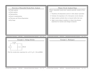
1. Example 1: Voltage Divider
31.25 nF
500 mHvg
vo
-
+
2 kΩ
Find the steady-state expression for vo(t) if vg(t) = 64 cos(8000t).
Portland State University ECE 221 Sinusoidal Steady-State Analysis Ver. 1.21 3
Overview of Sinusoidal Steady-State Analysis
• Nodal analysis
• Mesh analysis
• Superposition
• Source transformation
• Thevenin and Norton Equivalents
• Op Amps
Portland State University ECE 221 Sinusoidal Steady-State Analysis Ver. 1.21 1
Example 1: Workspace
Portland State University ECE 221 Sinusoidal Steady-State Analysis Ver. 1.21 4
Phasor Circuit Analysis Steps
Phasor (sinusoidal steady-state) analysis generally consists of four
steps.
1. Transform all independent sources to their phasor equivalent
2. Calculate the impedance (Z) of all passive circuit elements
3. Apply analysis methods that we learned earlier this term
4. Apply inverse phasor transform to obtain time-domain
expression for currents and voltages of interest
Portland State University ECE 221 Sinusoidal Steady-State Analysis Ver. 1.21 2

2. Example 3: Source Transformation
15 mH
v1
v2
vo
-
+
20 Ω
30 Ω 25/6 µF
Use source transformations to solve for the steady-state part of
vo(t). The sinusoidal voltage sources are:
v1(t) = 240 cos(4000t + 53.13◦
) V
v2(t) = 96 sin(4000t) V
Portland State University ECE 221 Sinusoidal Steady-State Analysis Ver. 1.21 7
Example 2: Current Divider
1 H
ig
io
50 Ω 250 Ω
20 µF
Find the steady-state expression for io(t) if
ig(t) = 125 cos(500t) mA.
Portland State University ECE 221 Sinusoidal Steady-State Analysis Ver. 1.21 5
Example 3: Workspace (1)
Portland State University ECE 221 Sinusoidal Steady-State Analysis Ver. 1.21 8
Example 2: Workspace
Portland State University ECE 221 Sinusoidal Steady-State Analysis Ver. 1.21 6

3. Example 4: Workspace
Portland State University ECE 221 Sinusoidal Steady-State Analysis Ver. 1.21 11
Example 3: Workspace (2)
Portland State University ECE 221 Sinusoidal Steady-State Analysis Ver. 1.21 9
Example 5: Node-Voltage Method
Vo
-+
5 Ω
j2 Ω
j3 Ω
-j3 Ω
5∠0◦
A 5∠-90◦
V
Use the node-voltage method to find the phasor voltage Vo.
Portland State University ECE 221 Sinusoidal Steady-State Analysis Ver. 1.21 12
Example 4: Kirchhoff’s Laws
Vg
Ia
Ib
Ic
5 Ω
15 Ω25 Ω
j25Ω -j15Ω
2∠45◦
A
The phasor current Ib is 5∠45◦
A.
1. Find Ia, Ib, and Vg.
2. If ω = 800 rads/s, write the expressions for ia(t), ic(t), and
vg(t).
Portland State University ECE 221 Sinusoidal Steady-State Analysis Ver. 1.21 10

4. Example 6: Workspace
Portland State University ECE 221 Sinusoidal Steady-State Analysis Ver. 1.21 15
Example 5: Workspace
Portland State University ECE 221 Sinusoidal Steady-State Analysis Ver. 1.21 13
Example 7: Node-Voltage Method
Vo
-
+
2.5 I1I1
8 Ω
j5 Ω
-j10 Ω 15∠0◦
A
Use the node-voltage method to find the phasor voltage Vo.
Portland State University ECE 221 Sinusoidal Steady-State Analysis Ver. 1.21 16
Example 6: Mesh-Current Method
Ib
Ia
Ic
Id
5 Ω
5 Ω
j5 Ω -j5 Ω
2∠0◦
A
50∠0◦
V100∠0◦
V
Use the mesh-current method to find the branch currents Ia, Ib, Ic,
and Id.
Portland State University ECE 221 Sinusoidal Steady-State Analysis Ver. 1.21 14

5. Example 8: Workspace (1)
Portland State University ECE 221 Sinusoidal Steady-State Analysis Ver. 1.21 19
Example 7: Workspace
Portland State University ECE 221 Sinusoidal Steady-State Analysis Ver. 1.21 17
Example 8: Workspace (2)
Portland State University ECE 221 Sinusoidal Steady-State Analysis Ver. 1.21 20
Example 8: Th´evenin & Norton Equivalents
a
b
1 Ω
12 Ω
12 Ω
12 Ω12 Ω
j12 Ω
-j12 Ω
87∠0◦
V
Find the Th´evenin and Norton equivalents of the circuit in the
phasor domain.
Portland State University ECE 221 Sinusoidal Steady-State Analysis Ver. 1.21 18

6. Example 10: Superposition
15 mH
v1
v2
vo
-
+
20 Ω
30 Ω 25/6 µF
Use superposition to solve for the steady-state part of vo(t). The
sinusoidal voltage sources are:
v1(t) = 240 cos(2000t + 53.13◦
) V
v2(t) = 96 sin(8000t) V
Portland State University ECE 221 Sinusoidal Steady-State Analysis Ver. 1.21 23
Example 9: Th´evenin & Norton Equivalents
b
a
0.02 Vo
Vo
-
+
40 Ω
600 Ω j150 Ω -j150 Ω
75∠0◦
V
Find the Th´evenin and Norton equivalents of the circuit in the
phasor domain.
Portland State University ECE 221 Sinusoidal Steady-State Analysis Ver. 1.21 21
Example 10: Workspace (1)
Portland State University ECE 221 Sinusoidal Steady-State Analysis Ver. 1.21 24
Example 9: Workspace
Portland State University ECE 221 Sinusoidal Steady-State Analysis Ver. 1.21 22

7. Example 11: Workspace (1)
Portland State University ECE 221 Sinusoidal Steady-State Analysis Ver. 1.21 27
Example 10: Workspace (2)
Portland State University ECE 221 Sinusoidal Steady-State Analysis Ver. 1.21 25
Example 11: Workspace (2)
Portland State University ECE 221 Sinusoidal Steady-State Analysis Ver. 1.21 28
Example 11: Operational Amplifiers
100 pF
50 pF
vg
vo
-
+
10 kΩ20 kΩ
25 kΩ
40 kΩ
Find the steady-state expression for vo(t) given that
vg(t) = 2 cos(105
t) V.
Portland State University ECE 221 Sinusoidal Steady-State Analysis Ver. 1.21 26

8. Example 12: Workspace (2)
Portland State University ECE 221 Sinusoidal Steady-State Analysis Ver. 1.21 31
Example 12: Operational Amplifiers
0.1 nF
vo
-
+
vg
20 kΩ
80 kΩ
160 kΩ
200 kΩ
Find the steady-state expression for vo(t) when
vg(t) = 20 cos(106
t) V.
Portland State University ECE 221 Sinusoidal Steady-State Analysis Ver. 1.21 29
Example 12: Workspace (1)
Portland State University ECE 221 Sinusoidal Steady-State Analysis Ver. 1.21 30