batch chemical reactor

1. Compurers them. Engng, Vol. 16, No. 1, pp. 2749, 1992
Printed in Great Britain.All rightsreserved
009%1354/92 $5.00 + 0.00
Copyright6 1992F’ergiunonPressplc
CONTROL OF AN UNSTABLE BATCH CHEMICAL REACTOR
G. E. ROTSTEIN and D. R. LEWIN~
Department of Chemical Engineering, Technion, Israel Institute of Technology, Haifa 32000, Israel
(Received 18 September 199O;final revision received 8 July 1991; received for publication 22 July 1991)
Abstrnct-As often experienced in industrial practice, a fixed-parameter PID can do a good job, even for
potentially challenging problems such as open-loop unstable processes. However in such cases, consider-
able a priori process knowledge may be required in order to adequately tune the controller and make the
control performance robust to changes in operating conditions. Adaptive schemes, on the other hand,
require less prior plant information but they should not be regarded as magic solutions to control
problems. In this study, alternative adaptive control schemes are presented for the temperature control
of an open-loop unstable batch chemical reactor in which the sequential exothermic reactions A-B-X
are carried out. The performance of such control systems are compared with that of a PID controller,
designed using IMC-based rules, and detuned to ensure robustness to process parameter changes along
the temperature trajectory. Since the required detuning results in poor disturbance rejection, one would
expect that the adoption of adaptive strategies should improve performance. However, the fact that u
fixed-parameter PID controller can be designed to perform reasonably well does not impiy that a self-tuning
version will do at least as well. A self-tuning scheme combined with a parametric control approach can
successfully deal with the reactor start-up and the regulatory problem, provided that the adaptive scheme’s
process model order is adequately selected. Thus, a self-tuning PID controller, which is based on a
second-order model, is liable to failure if the true process is effectively of higher order.
1. INTRODUmION
Batch reactors have been used for some time in the
pharmaceutical and fermentation industry and, to a
smaller extent, in the chemical process industry (e.g.
in exothermic polymerization reactions). However,
an increase in their application can be expected in the
future. When compared with continuous reactors,
they have the following main advantages: (i) batch
reactors are flexible, and can be adapted to small
production runs of various products; (ii) they present
less scale-up problems, allowing complex chemical
synthesis to be conducted essentially in the same way
as in the laboratory; and (iii) batch systems are better
suited to carry out reactions under sterile conditions,
and to deal with dangerous materials. The import-
ance of these considerations are apparent in a chemi-
cal industry moving in the direction of “expensive
chemicals” and which is greatly influenced by the
rapid changes in market demand and the advent of
new technology. On the other hand, the control of
exothermic batch reactors can result in an extremely
difficult regulatory problem. They usually present
strong nonlinear characteristics brought by the heat
generation term in the energy balance. Since the
process outputs must be controlled along a tem-
porally varying trajectory, steady-state operating
conditions do not generally exist, and process vari-
ables and parameters may exhibit large changes with
time. In addition, if the reactor is operating such that
~To whom all correspondence should be addressed.
it is open-loop unstable, control failures can lead to
thermal runaway.
A good review on problems and results in batch
reactor control was presented by Juba and Hamer
(1986). A variety of temperature control schemes
have been proposed as alternatives to conventional
feedback: a feedforward-feedback scheme (Jutan and
Uppal, I984), generic model control (Cott and Mac-
chietto, 1989), and many applications of self-tuning
and adaptive control techniques (e.g. Kiparissides
and Shah, 1983; Cluett et al., 1985). In all these
studies, the performance of the proposed control
scheme is compared with that of a PID algorithm,
although very little indication is given about how the
PID controller was tuned. Adaptive control is a
nonlinear strategy and significantly more complex
than a fixed-parameter PID scheme. It is therefore
valid to question whether comparable performance
could be obtained with the more traditional PID
feedback controller (AstrBm, 1983).
The start-up of exothermic batch reactors is par-
ticularly problematic because heat must be applied to
raise the batch to reaction temperature and then be
removed. This requires two manipulated variables
and generates an overdetermined problem with too
many degrees of freedom. In the adaptive strategies
proposed to date, the start-up problem has been
solved by working with a constant amount of cooling
and manipulating the heating rate (Kiparissides and
Shah, 1983; Cluett et al., 1985) or by employing a
heating bath at constant temperature and controlling
the cooling flowrate (Tzouanas and Shah, 1985,
27

2. 28 G. E. Ronram and D. R. LENIN
1989). Alternatively, the switching instant from heat-
ing to cooling in a dual-mode strategy has been
calculated based on an adaptive prediction algorithm
(Merkle and Lee, 1989). This particular method was
experimentally tested on a batch process with no
reaction, essentially a linear system. Prediction prob-
lems should be expected if the batch process involves
exothermic reaction. A parametric control approach
(Jutan and Uppal, 1984) was applied to implement a
feedback-feedforward scheme. Here, the number of
degrees of freedom is reduced by allowing both
manipulated variables to change through a single
parametric variable. Finally, an expert system
(Regev et al., 1989) that can learn the “best” start-up
strategy based on operating experience has been also
proposed as a possible solution.
This paper represents a full account of preliminary
results previously presented (Rotstein and Lewin,
1990) and has the following two objectives:
(A)
tw
The generation of simple systematic rules for
the tuning of PI and PID controllers for
open-loop unstable systems, and the definition
of stability limitations imposed by model
uncertainty. This will serve as a systematic
basis for comparison with more advanced
control strategies, and has not in general been
covered adequately in previous published re-
sults. These rules will help to avoid extensive
on-line tuning and serve as criteria to indicate
when upgrading the PID controller becomes
unavoidable.
To study the potential performance improve-
ments and the implementation difficulties
encountered in the upgrading of a fixed-
parameter PID scheme to self-tuning con-
trollers. It is natural to conceive of the idea of
replacing a conventional PID control scheme
by its adaptive version. Implementing such a
scheme would reduce the necessary tuning
efforts every time changes take place (e.g.
plant upsets, different reactions) and eventu-
ally, cope with the start-up problem. Several
manufacturers already market self-tuning PID
controllers which are clearly more acceptable
to the conservative chemical industry than
higher order schemes involving large numbers
of tunable parameters. Is this proposed tran-
sition so simple? On the basis of the results
presented by others, the consensus is that the
implementation of self-tuning control can
usually be made to work with relative ease. In
this work, a self-tuning PID scheme is intro-
duced for the control of a typical exothermic
batch reactor example. Two implementation
issues are studied which highlight the prob-
lematic associated with utilizing adaptive
schemes. The first one is the neglected dynam-
ics problem. It has been recently shown
(Ydstie, 1986) that in the presence of
model-plant order mismatch, even simple
linear systems under adaptive control can
exhibit very complicated dynamic behavior
(even chaos). The second issue concerns
the constraints imposed on the initialization
algorithm of the adaptive scheme by safety
considerations, which are specific to the
particular control problem.
2. TUNING FOR OPEN-LOOP UNSTABLE SYSTEMS
2. I. Objecrives
A design method has recently become available for
first-order unstable systems with time delay (De Paor
and O’Malley, 1989) where gain and phase margin
criteria are used. A more comprehensive approach
has been proposed (Quinn and Sanathanan, 1989)
but the resulting controllers cannot in general be
expressed in the three-mode PID form. The problem
of delineating the applicability of PI and PID
controllers for open-loop unstable processes with
parameter uncertainty was not addressed by either of
these studies. Simple tuning rules for PI and PID
controllers have been derived for open-loop stable
systems (Rivera et al., 1986) employing IMC (internal
mode control) as the design tool. In the present work,
the rules are extended for open-loop unstable sys-
tems. Tolerance limits for robust stability tuning
under gain uncertainty and unmodelled dynamics are
derived. The theory is tested on a nonlinear open-
loop unstable system, a model of a batch reactor in
which the exothennic consecutive reactions A-B-C
are carried out.
2.2. IMC controller design for open-loop stable and
unstable systems-a comparison
Control design is explicitly or implicitly a model-
based activity. An explicit model-based scheme could
be as sophisticated as a set of partial differential
equations describing the process solved on a real-time
simulator in parallel with the process. At the lowest
level of complexity, the use of “rule-of-thumb” tuning
rules for PI/PID controllers imply first- or second-
order lag approximations of the process. Clearly, the
quality of control will be intimately related both to
the sophistication of the process model and also of its
accuracy. However, even the most detailed model is
still only an approximation of reality, and an import-
ant property of the designed feedback controller is
that it be insensitive to modelling error. The relation-
ships between designed controller sophistication,
model uncertainty and achievable closed-loop per-
formance can be elucidated by using the concept of
IMC (Morari and Zafiriou, 1989).
The IMC design procedure utilizes the structure
shown in Fig. la, in which p(s) represents the “true”
process, p(s) is the process model and q(s) is the IMC
controller. After defining the model, the design of
q(s) consists of two steps. Firstly, the nominal con-
troller, q’(s) is computed in terms of the proposed

3. Control of an unstablebatch chenricalreactor 29
linear model, thus tacitly assuming that it is accurate.
The second step is to append a low-pass filter, f(s)
[q(s) = Q(s)f(s)], in order to attenuate the effect of
model uncertainty, which usually increases with fre-
quency. This has the effect of detuningthe controller,
or in other words, reducing the controller gain.
For open-loop unstable systems, the IMC structure
shown in Fig. la is internally unstable and thus can
only be utilized as a design tool. The parametrization
for the feedback classical controller:
q(s)
c(s)=[1 - P(s)q(s)] ’
is used to effect the implementation in the classical
control structure, shown in Fig. 1b.
Theorem-Robust stability (Morari and Zafrou,
1989)
The closed-loop system is robustly stable if and
only if the controller stabilizes the nominal plant d
and:
1
If( c--_, VW. (2)
&l(o)
Wheref(s) is the IMC filter and z(s) is the upper-
bound multiplicative uncertainty:
I,(o) 2 Ik(w)l =
I”
(iw) -j?(k)
NW)
7VW, VP E n, (3)
where II defines the set of all possible plants in the set:
n = {P(S) IP(S)
a,s”+a,_ls”~‘+...+a,s+~e_8,
= b,s”+b,_,.F’+-..+b,s+l >
1 (4)
When following the IMC design procedure, the differ-
ences between open-loop stable and unstable systems
arise in the selection of the IMC filter. For stable
Disturbance
Setpoint output
(a>
Disturbance
setpoint output
(b)
Fig. 1. (a) The IMC feedback structure. (b) The classical
feedback structure.
processes, the only condition imposed on the filter
f(s) is that it be unity at s = 0, which will ensure
offset-free response. For unstable processes, the filter
f(s) must in addition be unity at the location of all
the unstable poles of the nominal model. The follow-
ing important consequences from a robust stability
point of view can be derived:
2.2.1. Open-loop stable systems. If the uncertainty
in the steady state gain is under 100% we can always
guarantee the existence of a robust feedback con-
troller that can achieve zero tracking error for step
inputs. In such cases, the IMC titer is a low-pass filter
usually selected to be of the form:
1
f(s) = (& + 1)“’
where n is selected to ensure proper controller. For
robust stability there exists a trivial solution in A-+ co
(open-loop conditions). When tuning we must simply
increase the value of 1 until condition (2) is satisfied,
leading to a more sluggish response. Thus, there
exists a minimum value of A (&,) that provides
robust stability for the given level of model uncer-
tainty. If we in addition specify some performance
requirement, this is equivalent to imposing an upper
limit on A (A,). Excessively high performance spe-
cification will clearly be unattainable if A_ < &,.
2.2.2. Open-loop unstable systems. For open-loop
unstable systems there exists no trivial solution.
Robust stability cannot be guaranteed by simply
increasing A since a minimum amount of feedback
compensation is needed to avoid instability. Low-
frequency (gain) uncertainty considerations will
impose an upper limit on R (A,,), while high-
frequency uncertainty (unmodelled dynamics) will
limit its minimum value (&,)_ If the amount of
uncertainty is too high, there may exist no controller
that can guarantee robust stability and a better
model (less uncertainty) is required. Thus, the robust
stability problem for open-loop unstable systems is
of the same degree of complexity as the robust
performance problem is for stable ones.
2.3. IMC-based PI and PID tuning rules for open-
loop unstable systems
When tuning according to the IMC design pro-
cedure for step inputs and nonminimum phase un-
stable processes, equation (1) is reduced to:
1 f
c=3(1--f)
a simple form for the IMC filter f(s) for first- and
second-order open-loop unstable processes is (Morari
and Zafirou, 1989):
ys + 1
f(s) = (h + I)2 ’
y=A 1+2,
( >‘c”
(7)

4. 30 G. E. ROT-STEIN and D. R. LEWIN
Table 1. IMC tuningrules.for PI and PID controllers [y = I(I/fu + 211
P(s) J-(s) KC% 71 %I
Kp YS + 1
-y
Y 0
-7.9 + 1 (A.9 + 112
K* ys + 1 _dY + q31) YTpl
(--+.s + l)(s.,s + 1) (As + 112 12 Y ++p1
Y++.I
where 7” is the unstable time constant of the model.
The tuning rules derived by substituting f(s) and y
from equation (7) into (6) are summarized in Table 1.
Here we present tuning parameters for a theoretical
PID algorithm, which is improper (it has two zeros
and one pole, and is therefore unrealizable). If a
third-order filter is employed using a second-order
model, a proper PID (augmented by a lag) would be
obtained.
For open-loop stable systems, I appears solely in
the controller gain and changing K, is an adequate
tuning method (Rivera et al., 1986). For unstable
open-loop processes, simultaneous changes in all the
control modes are needed. We note that IMC tuning
parameter jl appears in all the controller coefficients,
explaining the dificulties encountered in tuning con-
trollers for this type of process. The IMC design
approach reduces the problem to a 1-D parameter
search in both cases; it also provides a robustness
analysis method for the tuning of controllers in the
presence of model uncertainty.
2.4. Robustness anaIysis
The tuning rules presented in Table 1 will be of
limited practical use if they are not accompanied by
an adequate robustness analysis method. When the
modelling error is described in terms of the multi-
plicative uncertainty defined in equation (3), the true
uncertainty regions in the Nyquist plot are approxi-
mated at each frequency by disk-shaped regions. A
design based on this approximation can add conser-
vativeness to the controller tuning. For open-loop
stable systems, this additional severity does not seem
to be particularly critical (Laughlin et al., 1986).
However, for open-loop unstable systems, it can be
shown (see Appendix A) that PI and PID controllers
tuned according to the IMC-based parameters cannot
satisfy the robust stability criterion based on multi-
plicative uncertainty when gain uncertainty is greater
than 87%.
In order to check the conservativeness introduced
by the disk-shaped regions, the Routh-Hurwitz
method was applied to a process in which there is
gain uncertainty and in which one stable pole is
neglected in the model:
P(s)= K-----P(s),
(7s + 1)
K = K,/&,, K,GK,GK,. (8)
Following the rules given in Table 1, it is obvious that
in order to generate a PI controller, p”(s) must have
one unstable pole only, while for a PID controller, it
must have one stable and one unstable pole. In
Appendix B, we prove that when there is no dynamic
uncertainty (i.e. no neglected poles and flxed, known
time constants), robust PI and PID controllers can
always be tuned if there is no change in the sign of
the process gain Kp. The limit on the level of gain
uncertainty previously found is thus an artifact intro-
duced by the conservativeness of the multiplicative
uncertainty robust stability condition.
Restrictions on gain uncertainty (defined as 11- K I)
and r-values are also demonstrated in Appendix B.
The time constant of the neglected pole z must always
be smaller than the time constant of the unstable
pole. The results are summarized in Fig. 2 where
11 -Kim, is plotted as a function of A./r, for different
values of r /7,. From the graph, the permitted range
of 1 can be obtained given the levels of dynamic and
gain uncertainty. This delineates the conditions in
which robust stability cannot be guaranteed using PI
or PID controllers. This is a particularly interesting
result, because it indicates cases in which these tra-
ditional controllers cannot work and more advanced
strategies (e.g. adaptive, which reduces the amount
of effective uncertainty by continually updating the
process model) would become unavoidable.
3. APPLICATION TO THE CONTROL OF AN
EXOTHERMIC BATCH REACTOR
Thus far, the results obtained have been of a
general nature, and could be applied to any minimum
phase process which has one unstable pole. We shall
now apply these results to a specific example, that of
Fig. 2. Robust stability range for PI and PID controllers in
the presence of gain uncertainty and neglected dynamics.
The figure shows contours in the (A/r,, 11- K I,,) planefor
differentvaluesof T./T,(0.0-0.7).

5. Control of an unstablebatchchemicalreactor 31
a batch exothermic reactor. The study will qualitat-
ively illustrate the method and indicate the achievable
performance obtained using conventional PI/PID
controllers. These results will later be compared with
the performance of adaptive schemes.
3.1. Mathematical model
In a typical batch reactor, steam is used to raise the
reaction temperature to the desired level after which
cooling water is used to remove the heat of reaction.
For the example process used in this study, the
reaction system is the two consecutive first-order
reactions:
Akl-B&C. (9)
The mathematical model presented below is based on
that given by Luyben (1973). The heating and cooling
mechanisms have been simplified. Instead of intro-
ducing a two-phase model to account for steam and
water in the jacket, we shall assume that the cooling
and heating fluids in the jacket are of equal density
and heat capacity (which are independent of tempera-
ture) and that the jacket is always filled. These
measures remove several state variables and also
reduce the description of heat transfer from the
jacket to the wall to one coefficient. These modifi-
cations do not remove the significant elements of
the problem and allow us to focus our attention to
the main issues. The simplified mass and energy
balances are:
dC,
dr=
-k,C,, k, = a, exp(Ea, /RT), (10)
dCB=_kC -kc
t 1 A 2 B, k2 = a2exdEa21RT), (11)
dT k, (TX,4 + k,G?G4-=
dt PC,
+ h,(T, - T),
(12)
(13)
dT,_ MT, - T,) - h, (r, - T)
dt - 8,
(14)
The initial conditions were assumed to be those
supplied by Luyben (1973), and are listed in Table 2.
Table 2. Initial loading conditions
Variable Value (example) Value (s.i. units)
T 80°F 300K
TlIl 80°F 300 K
7J 80°F 3OQK
G 0.8 lbmol A ft-”
c. 0.0 lbmol B ft-’
12.8 kgmol mm3
0.0 kgmol m -’
T, 80°F 300K
Th 260°F 400K
Variable
Table 3. Design parameters
F0llYXllatioIl Nominal value &xamulc)
e2
3 x lo-‘s-1
0 F-
V,
I8 x IO-‘s-’
The nominal values of the design parameters which
appear in Table 3 were computed from data supplied
by the same source. Assuming pseudo-steady-state
in the concentrations and linearizing around the
followed trajectory (see Appendix C) the system can
be modelled as:
T(s)
p(s)=----= -s
U,(s) (-GS + 1) (q.lS + 1)(z, + 1)’
W)
where T(s) is the reactor temperature, U,(S) rep-
resents the coolant flow, rU is the time constant
corresponding to the unstable pole and T,,~and rpzare
related to the time constants for transients in coolant
temperature and reactor walls, respectively. Along
the desired trajectory, we can calculate the variation
on the linear model parameters from the moment the
state derivatives approximate to zero until the end of
the reaction. In this way, the following uncertainty set
is obtained:
94 < Kp c 1396,
1368<z, <3516s,
168<2,,<57Os,
T $ z= 50 s (16)
and the nominal parameter values are: $ = 745,
f,, = 2442 s and zip,= 372 s.
3.2. PI and PID tuning simulation results
3.2. I. Robust PI control. We will first check the
possibility of controlling the batch reactor under
study using a PI controller. To tune a PI controller
as suggested in Table 1, the two stable poles of the
Table 4. Kinetic parameters
Value
Variable Nominal value (s.i. units)
a1 729.55 min ’ 12.16s-’
2
6467.6 min-’ 109.5 s-1
EL2:
- 1.5 x lo4 B.t.u. mol-’ -3.48 x lO’kJmol-
-2 x lo4 B.t.u. mol-’ -4.64 x 10’ kJ mol-’
A, -4 x 1O’B.t.u. mol-’ -9.28 x lO“kJmo1-’
A, -5 x 10’B.t.u. mol-’ - 11.6 x lti kJ mol-’

6. 32 G. E. ROTSTEIN and D. R. LEw~N
system are neglected. The following nominal model
and controller parameters are obtained:
B(s) =
-745
-2442s+l
& = 3.3y In= and rr=y . (17)
The value of R is selected based on robust stability
considerations or can be tuned on-line. However, in
the present case, 0.07 < ~~,/f,, c 0.23, and according
to the robustness criteria obtained in Appendix B
and summarized in Fig. 2, if the time constant of
the dominant neglected pole is of the order of 20%
of the nominal unstable time constant, the maximum
gain uncertainty that can be tolerated is 80%. In the
particular application under study:
K---W
gain uncertainty = 100 y = 87%.
I IP
We can therefore conclude that a PI controller cannot
be designed to guarantee robust stability. This analy-
sis has assumed that the effect of the fast pole (at
7p2 u 50 s) is negligible. It is thus a subset of the
original uncertainty set given in equations (15) and
(16). If no PI controller can be robustly tuned for this
subset determined by gain and neglected dynamics
uncertainty only, there will exist no robustly tuned
PI for the complete set. By opting for a PID con-
troller design, the neglected dynamics uncertainty
is reduced and this increases the level of gain
uncertainty tolerated.
3.2.2. Robust PID controller. In order to obtain a
PID controller, only the fast stable pole (Tag) must be
neglected. From Table 1 we obtain the following
control parameters:
- 745
‘(‘I = (-2442s + 1) (372s + 1)
4 3 3 (Y += 372) ;
A2
7,=(372+A) (18)
3727
‘c = (372 + y)’
The IMC filter has the same form as in the PI case.
In this case, sVZ/TUis close to zero and as shown in
Fig. 2, there is virtually no limit on the level of gain
uncertainty. Thus, for this particular set of conditions
and ignoring dynamic uncertainty, a PID controller
can always be tuned for robust stability. The use
of Fig. 2 might be particularly useful when gain
uncertainty dominates and when the tuning of the
control parameters is performed directly on-line. The
existence of a working range of ;i for the actual
uncertainty set (16) will now be checked. In Fig. 3,
the robust stability test defined by equation (3) is
executed for a PID controller. Here, the conservative
multiplicative uncertainty bound eliminates the possi-
biiity of employing PID control. Tuning with the
actual Nyquist uncertainty regions has been proposed
as an alternative method (Laughlin er al., 1986) in
order to reduce the conservativeness of the robustness
test. In order to guarantee robust stability, the follow-
ing conditions must be satisfied:
Condition 1.
Condition 2.
The nominal system (p =p) must
be stabilized by the controller. In
this case, p(s)c(s) must do one encir-
clement of (- 1,O) in the anticlock-
wise direction.
At each frequency w, the uncertain
process p(s) E II is contained by the
region A(W) in the complex plane.
The regions n(o)c(iw) must also
encircle and exclude ( - 1,0) for all
frequencies w.
The implementation of this robustness test is clearly
more time-consuming than that based on multiplica-
tive uncertainty. The additional effort is only justified
when working with the approximated disk-shaped
regions is excessively conservative and makes design
impossible. The computation of a range of ;i which
satisfies robust stability involves a lengthy trial-and-
error search in which the uncertainties in all the
parameters in the set (16) are included. The feasible
range of filter parameter values which guarantee
robust stability when only gain uncertainty and one
neglected pole are considered (from Fig. 2, this range
is rlE [30, 7201, with time in seconds) will clearly
bracket the range of I when time constant uncertainty
is also to be accounted for. The range obtained from
Fig. 2 can be used as a bound for the search for filter
parameter values that guarantee stability for the plant
defined by equation (16), the final result being the
range: A E [60,480].
The conservativeness added by the multiplicative
uncertainty test can be clearly observed in Fig. 4,
where the test has been plotted for A = 240 s. The true
uncertainty regions encircle the point (- 1,O) once in
the anticlockwise direction (thus satisfying the
Nyquist stability criterion, since there is one positive
pole) without including it for any value of o. On
the other hand, the disk-shaped regions completely
envelope the point leading to the failure of the robust
stability test (Fig. 3). The additional severity added is
particularly critical in this case, because it would
reject simple PID feedback for the control of the
batch reactor temperature.
Simulations were performed with the PID con-
troller tuned according to equation (18) with a value
of A = 240 s (in the center of the permitted working
range). A dual-mode start-up strategy (Shinskey,
1979) was adopted. The results are presented later
for performance comparison with the implemented
self-tuning schemes. We will now turn our attention
to a brief review of the design theory for simple
adaptive controllers.

7. Control of an unstable batch chemical reactor 33
1.25-
l-
Lm-
30
Frequency (Rad/minl
Fig. 3. The robust stability condition based on multiplicative uncertainty. Shown in the figure is the
frequency-dependent magnitude of the IMC filter f(s) given as equation (7) for 1 = 0.1. 1 and 10 min
(respectively) as well as the multiplicative uncertainty bound F.
4. ADAPTIVR CONTROL
An adaptive control scheme can be defined as any
regulatory strategy which can change its behavior in
response to changes in the dynamics of the process or
disturbances (Astrom, 1983). An adaptive scheme
performs two tasks on the system to be regulated: (i)
on-line parameter estimation (model identification);
and (ii) control law updating. Three distinct ap-
proaches can be identified: gain scheduling, model
reference control and self-tuning algorithms. We
have opted to apply a self-tuning technique based on
pole placement design which leads to controllers of
arbitrary order. This can be considered as being
composed of two loops: the inner loop consisting of
an ordinary linear feedback controller, and the outer
one composed of a recursive parameter estimator and
a design calculation rule (pole placement) which tunes
the internal control law according to the identified
parameters. This approach can lead directly to con-
trollers with PI or PID control structures. Perform-
ance is specified in terms of the desired location of
closed-loop poles and zeros.
4.1. On-line parameter estimation algorithms
The parameter estimation algorithm is the heart of
any adaptive scheme, and must be efficient and easy
to implement (low computation time requirements).
Recursive parameter estimation schemes are a class of
on-line identification methods which are particularly
attractive. Here, current values of the model par-
ameters are calculated as a function of the previous
estimations and the actual values of the inputs and
outputs of the system. Common to these algorithms
is the model assumption that supposes the system
2,
2 1
-._:.--..*s
:~=o.os‘=..
0
1,_, _.... ...‘... ,,,, _~
___“-A
.-_
--_-_--___+--- ---4 wzc6‘l
-1
_ _,c:;;
K, disk for a= 0.:
I
-8 -7 -6 -S -4 -3 -2 -1 0
R&l 2
Fig. 4. Nyquist uncertainty regions and multiplicative uncertainty disks. Shown in the figure are: (i) three
representative uncertainty regions for the process modelled as equations (IS) and (16), at w = 0.05. 0.1
and 0.5 rad mm-‘; (ii) uncertainty disks computed on the basis of multiplicative uncertainty, of which only
that for w = 0.5 rad min-’ appears on this scale; (iii) the plot pc(iw), where j is the reduced second-order
model appropriate for PID design [equation (18)l.

8. 34 G. E. Rorsrxr~ and D. R. LEWIN
can be represented by a deterministic autoregressive
moving-average (DARMA) model:
where n is the number of poles and m the number of
zeros in the model. One of the most widely used
estimators is the popular recursive least squares
(RLS) algorithm (Goodwin and Sin, 1984).
4.2. Recursive least squares (RET) algorithm
The RLS algorithm can be expressed as:
6k=6k-,+ Pk-24k-1
1 +dZ-,pk-*4k-,
(Y*-4L,&-,)9
(20)
Pk-_I = P&2 -
Pk-24k-l4~-lPk-2
1 +&E-,PPk--2#Jk-, ’
(21)
where Pk is the covariance matrix, & is a vector of
model parameters and c#J~_., is a vector of previous
inputs and outputs: r#~_ I = [y(k - 1), Y(k - 2), . . .
y(k -n), u(k - 1), u(k - 2), . . . u(k -m)]. The in-
itial conditions are: 8, and P_ 1= P,,, where PO is
an arbitrary positive-definite matrix. Usually, we
take P,, = ~1, where K is a positive constant. Several
variations on the RLS have been proposed for
the identification of time varying systems, namely
the covariancc matrix resetting algorithm and the
exponential “forgetting factor” method (Fortescue
et al., 1981). Both of these alternatives aim at pre-
serving adequate sensitivity of the identification
algorithm.
4.3. Pole placement control law
Pole placement is a simple design procedure which
is well described in the literature (Astrom, 1983). A
feedback law is generated so that the identified model
has the desired closed-loop poles and zeros. In the
first part of this work we noted that the linear model
approximation for the reactor temperature response
to changes in cooling and heating flow is essentially
of third-order. Therefore, the pole placement algor-
ithm for a third-order DARMA model is first
described.
4.4. Pole placement based on a third-order model
We assume a third-order linear model of the form:
We want to find a feedback law such that the
closed-loop system has the poles of a continuous
system with the characteristic polynomial:
(s2 + 2&s + 02) (73+ 1) = 0. (23)
This means that the required closed-loop discrete
characteristic polynomial should be:
A,(z-‘) = 1 + a,,~-’ + u,zV2 + a,sz-‘, (24)
where
a,,,, = [2 exp(-<oh) cos Jm + exp (h/z,)],
%I2 = exp( - ewh)[2 exp(h/r,) cos ,/-
+ exp( - twh)l,
a,, = exp[ - (2&h + h /T3)1.
Tuning the control law is effected through the selec-
tion of four parameters: h, the sampling interval; <.
the damping coefficient; CIJ,the natural frequency (or
desired bandwidth) and T,. If the two zeros which
appear in B(z -I) in equation (19) correspond to
poorly-damped modes, they cannot be cancelled by
the controller [see the discussion in Wittenmark and
Astrom (1980)]. A new desired denominator P,,, is
defined in order to cancel the plant zeros only when
it is considered useful to do so:
P,(z -1) = A,(z-‘)B+ (I -1) (25)
and B, (z-l) contains only the well-damped zeros of
the denominator that are to be cancelled. The control
law is:
Ru, = 5, - SY,, (26)
where we choose:
T = s, + s, + s* + sj.
According to the internal modelprinciple (Francis and
Wonham, 1976), in order to introduce reset in the
controller, we define R(z-‘) as:
R(z-‘)= R,(z-‘)(l -z-i)
=(l+r,z-‘+rz~-~)(l -z-l). (27)
To obtain the control law parameters the Diophan-
tine equation must be solved:
A(z-‘)R,(z-I)(1 -z-‘)+z-‘B(z-‘)S(z-‘)
= P,(z-‘). (28)
This equation can be expressed as a system of linear
equations and requires the inversion of a 6 x 6 matrix
for its solution.
4.5. Pole placement based on the PID form @oUowing
Wittenmark and AstrCm, 1980)
A self-tuning PID control algorithm can be derived
if a second-order DARMA model is assumed in
equation (19) (us = b, = 0), in which case r, is selected
as zero. When these values are introduced in equation

9. Control of an unstable
(23) and the parameters for R, are calculated,
there is a zero present at - b2/b, and B, is defined
as:
B+(z-,)= [(l+$z-‘) -0.1< +0.99, (29)
[
1 6, 0
a, - 1 b2 4
a2 - ai 0 b2
--a2 0 0
[;]+EY$:].
(31)
1 1 otherwise
and P,,, has the form:
P,(z--1) = 1 +p,,z-r +~,2z-2+pmrZ-3, (30)
where
Pm1=%I1 --z,,
Pm2 = am2 - amI z,,
pm3 = ---a,2z,,
{
62
z,(z-‘) = -b,
-0.1 < $< 0.99,
I
0 otherwise.
Thus s, = r2 = 0 in equations (27) and (28) and
the Diophantine equation solution (28) requires the
inversion of a 4 x 4 matrix:
At each sample interval, the parameters of the poly-
nomials A and B are obtained from the identification
algorithm and we then perform the inversion of the
above matrix in order to calculate the four control
law parameters.
4.6. Translation to PID parameters
Several different structures can be proposed for a
classical PID controller in sample data from (Astrom,
1983). If no additional filter is added to force the
controller to be proper, the following incremental
form may be stated.
+(I+?>,-I )-+-2 . (32)
For the special second-order case detailed above, the
control law can be expressed as:
(1 +rlz-L)(l-zZ-‘)~k_l=(l +r,z-‘)Auk
= Ty,--Soy,--sly,-, --s2yk-2. (33)
Comparing the last two equations we can easily
identify equation (33) as a classical PID controller
with an additional filter on Au,. This fllter, that
batchchemical reactor 35
makes the controller proper, has an “optimal” time
constant r, in place of being a simple function of ‘cn.
The relation between &, r,, 7,, and s,, si, s, can be.
found now by simple comparison of the two control
laws.
K, = - (s, + 2s, ).
7D s2
-= --*
h K,
71 s, + s, + s2
-=-
h K .
4.7. Conditions to avoid the additional fiker
As we have seen when a complete second-order
sampled-data model is employed, a PID with a filter
on Au, is obtained. If we assume a second-order
model with no zero (b2 = 0), a PID traditional non-
proper structure is derived. The algorithm design is
now:
A(z-‘)= 1 +a,~-i+a~z-~
B(z-‘) = b, 1
(34)
and P,,, = A,,, because of the absence of zeros to be
cancelled. Solving equation (31) for this particular
case (A, = P,, b, = 0) gives:
r, = 0;
s,=(Pl+ 1-al).
b, ’
s
L
= (P2 + a1 - a21 ;
b,
s2=a,.
b,
(35)
By substituting these values into equation (33), the
following three-mode control law is obtained:
A%= TY,--oY~-I--~Y~-~~ (36)
which corresponds to the well-known nonproper PID
structure.
4.8. Selection of the control tuning parameters
The selection of the desired closed-loop poles is
equivalent to tuning in conventional control schemes.
In the case of the self-tuning PID shown above, it is
important to provide a clear and simple tuning
procedure. In the absence of such, the control per-
formance attained could only be marginally better
than that obtained using fixed-parameter controllers.
The three tuning parameter values are selected in the
following manner. The first step is usually to choose
the sample interval h taking into account the expected
time constants from previous experience with the
system (e.g. known necessary start-up time). Next, <
is selected (a typical value is 0.7). Only the bandwidth
w then remains to be adjusted. This parameter is a
measure of the confidence we have on the accuracy
of the process model. It is equivalent to I --( in
the IMC design method (Morari and Zafirou,
1989). Wittenmark and Astrom (1980) proposed the

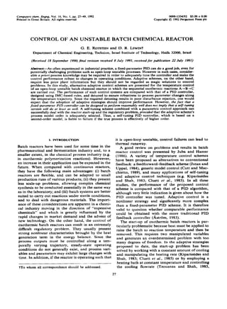
10. 36 G. E. R~TSTEINand D. R. LEWIN
following relationship to estimate an initial value
for w:
27t
o =N,hm
NC= lo-20
1
.
(37)
Subsequently, fine tuning must be carried out on-line
until a satisfactory response is achieved. As in fixed-
parameter controller tuning, increasing the band-
width provides a faster response but reduces
robustness and increases sensitivity to noise. For the
case of a third-order controller, both o and r3 must
be selected. This is the major drawback of higher
order models in adaptive schemes: the tuning activity
is increased. The computational task for the control
law is also heavier; there are six parameters to be
estimated and a 6 x 6 matrix to be inverted.
5. SELF-TUNING PID CONTROL OF A EXOTHERMIC
BATCH REAmOR
5.1. Confrol variable definition-the start-up problem
Exothermic reactions can pose a significant control
problem because often heat must be supplied to raise
the batch temperature to attain reaction ignition and
then be removed. This requires two manipulated
variables and generates an overdetermined problem
with too many degrees of freedom. For our adaptive
scheme, a parametric control approach (Jutan and
Uppal, 1984) was considered promising. The number
of degrees of freedom is reduced by parametric
combination of the two manipulated variables. This
approach provides a smooth transition from heating
to cooling and avoids the hard switch point definition
characteristic of bang-bang strategies or the larger
start-up time and waste of energy introduced by
working with one of the utility fluid flows at a
constant value. As a drawback, heating is still em-
ployed along the entire batch cycle. Two manipulated
variables are available in our system: UC and U,,.
Through the artificial variabte Z, we can propose a
parametric representation of both control variables:
U,=a,Z -k/3,
>Uh=a,Z+B2 ’
(38)
Z is a parametric variable which by definition lies in
the range: 0 d Z -c Z,, . In this case, a linear func-
tion has been selected for simplicity but more compli-
cated nonlinear forms could also be employed (Jutan
and Rodriguez, 1987). We defme Z = 0 as the control
extreme where cooling is maximized (heating is set to
zero) while Z = Z,, represents the extreme where
heating is maximized (cooling is set to zero). Thus,
equation (38) becomes:
“mu
19
Z
u,=-
zmsx
aaxis selected as 2 in order to preserve the control
range of both manipulated variables. Past values of
Z will be the input of the linear model in the
identification algorithm. The control law should
provide the changes to be done in Z (AZ) which
are translated by equation (39) to variations in the
physical manipulated variables UC and U,,.
5.2. Initialization of the algorithm
A method to ensure a rapid start-up is necessary
when poor information on the model parameters is
available. In the present application, maximum heat-
ing (Z = 2) is applied for several control steps
(defined as the initialization period, z’) until sufficient
information is accumulated for an adequate esti-
mation of the parameters. From then on, the control
of Z is transferred to the proposed control law with
the desired working temperature as the set-point.
A safety analysis is required to guarantee that this
can be implemented with no risk. Useful design
parameters for temperature trajectory design in
exothermic batch reactors have been recently pro-
posed (Lewin and Lavie, 1990). Two characterization
times have been defined for the reactor start-up:
Minimum “feasible” start-up time, rb-This is the
time necessary to heat the reactant mass up to the
reaction temperature at maximum heating rate
(Z = 2).
Safe start-up time, rc-This is the time necessary to
heat the reactant mass up to reaction temperature,
guaranteeing at all times that cooling capacity
exceeds the maximum heat generation rate.
When z hand zc are plotted as a function of the jacket
space velocity, there is a value of @ (defined as the
critical safe jacket space. velocity, CD’) for which
zc = th (Fig. 5). When Qi z GS we can define a non-
hazardous initialization period ti such that:
ri > tC(from the definition of r’),
ti -z th (stop maximum heating before reaching
reaction temperature).
If the reactor is operating with @ -z CD*,the design of
a safe initialization algorithm becomes more com-
plex. If too much heating is applied at start-up, it is
@(rnif’)
Fig. 5. The definition of safe jacket space velocity 0’.

11. Control of an unstablebatchchemicalreactor 37
possible that there will not be sufficient cooling
capacity later in order to remove heat generated and
the reactor could go into uncontrolled thermal run-
away. An alternative initialization procedure for this
case will be proposed later.
For the exothermic reactor model under study, the
parameters are given by Lewin and Lavie (1990): at
nominal operating conditions @* ‘u 0.006 s-l. For the
nominal jacket space velocity 0 = 0.018 s-‘: zc < 60 s
and Thu 1200 s. Thus if the initialization period of
seven control steps (t’ = 840 s at a 120 s sample
interval) is selected, r’ satisfies the safety conditions
previously defined.
5.3. Tracking changes of the linear model parameters
Two methods to preservetheidentification scheme’s
sensitivity to changes in the identified parameters
have been mentioned: covariance matrix resetting
(Goodwin and Sin, 1984) and variable forgetting
factor (Fortescue et al., 198 1). Both of these methods
were tested by simulation as a part of the self-
tuning PID algorithm as applied to the batch reactor.
Even though the resulting performances achieved
when adequately tuned weresimilar, covariance matrix
resetting was selected because it was more easily
tuned than the variable forgetting factor algorithm.
For the RLS with covariance matrix resetting, the
essential tuning parameters are the instants when
reset must be performed. At first, a fixed resetting
period was selected but this approach is arbitrary and
introduces unnecessary oscillations in the control
variable. This was replaced by a more successful
alternative in which a supervisory procedure was
employed to assess when resetting is required. The
behavior of the jacket temperature rj is employed
as a measure of the control performance. When
the mismatch between model and system becomes
significant, this manifests itself by the appearance of
oscillations in the jacket temperature, indicating that
the control tuning has become inadequate. Failure to
retune the controller at this point could result in the
propagation of oscillations to the reactor temperature
itself, possibly leading to a total loss of control of the
system. Thus, the supervisory procedure continu-
ously monitors the jacket temperature. It will invoke
the identification scheme whenever the amplitude of
the jacket temperature relative to its baseline value
6q exceeds a prespecified limit 6TFIM (a tunable
parameter). The identification scheme will be kept
operational until the control is deemed adequate, as
indicated by two successive samples of STj below the
limit ST,fl” In addition, the supervisory procedure
can be summarized by the following rules:
Here, ST,(k) is the absolute deviation of the jacket
temperature from some base level at sampling instant
k. This is computed using a first-order autoregressive
filter:
Tj(k) = eq(k - 1) + (1 - a)q(k)
where
6q(k) = ITj(k) - Tj(k)l and L = 0.8. (41)
The supervisory procedure is based on the idea “If it
works, don’t touch it” (do not reset the control law
parameters if the closed-loop performance is ade-
quate). Indeed. experience showed that it was useful
to disconnect the identification algorithm in those
periods when only poor dynamic information is
available from the system. Even though there is
a tuning effort required by the procedure for the
selection of the maximum peak permitted, a rather
transparent concept is involved with a clear physical
meaning. A value of c5TpM= 5.6”C (10°F) was
found to give satisfactory results. The initial con-
ditions for the RLS algorithm are: g(O) = [O,0, 0] and
P(-l)=?Cz, K = 100.
6. SIMULATION RESULTS AND DISCUSSION
6. I. Self-tuning PID controller
The self-tuning PID control scheme described
above was applied to the simulated batch reactor.
White noise with a maximum magnitude of 0.55”C
(1°F) was added to the temperature signal in order
to make the control conditions in the simulation
more realistic. The self-tuning PID algorithm with
no additional filter was implemented first, with the
results shown in Fig. 6a. No covariance matrix
resetting was introduced on the RLS. Even though
acceptable performance is achieved at start-up, after
7500 s the jacket temperature begins to oscillate and
eventually, the oscillations propagate to the reactor
fluid temperature. The performance of this self-
tuning controller is far inferior to that obtained with
the robustly tuned PID controller (see Fig. lOa). If
the simulation is extended above the time of practical
interest (e.g. 5-6 h), the oscillations become definitely
unstable. The bandwidth selected was 0.3 min-*.
Further reduction of w is of little help.
As a conclusion we believed resettingwas necessary
in order to improve the quality of the model and as
a result upgrade the tuning of the controller. The
simulation results brought in Fig. 6b were obtained
incorporating the supervisory procedure [equation
(40)] to choose reset instants. No improvement was
If (ST(k) > 6Ty”) && (IDENTIFICATION = =OFF)
I
RESET(P) and CONNECT (IDENTIFICATION) 1
If {(6T,(k) c STy”) and (6q(k - 1) < sTfr”)}
DISCONNECT (IDENTIFICATION)
J

12. 38 G. E. ROT-STEINand D. R. LEWIN
(0)
400
G
_ 375-
T
if
3 350 -
iY
K
$ 325 -
k-
I I I I
2400 4800 7200 9600 1.
Time [ seconds I
-
Y
- 375
a,
5
> 350
0
k
a
z 325
+i
300
0 2400 4800 7200 9600 12
Time Iseconds)
w.
I
20
Fig. 6. The response of a self-tuning PID controller in nominal operatingconditions: (a) without
covariance matrix resetting; and (b) with covariancematrixresetting.
attained and indeed, from the first reset instant
(t = 3000 s) the performance deteriorates completely.
Since the identification scheme based on a second-
order model is not adequate, a possible explanation
might be the inappropriate choice of model order (the
model assumption).
6.2. A simplier case: first-order dynamics on T,
In order to look for the origin of the problem and
suggest possible solutions, a simpler case was studied.
The energy balance equation on the jacket [equation
(13) in the reactor model] was replaced by arbitrary
first-order dynamics on T,:
dr,=l
dt J
;(w- rj), (42)
where Tj, is the manipulated variable. Even though
this is not realistic from a physical point of view, it
allows independent manipulation of the jacket pole
location. Simulations were performed beginning with
low values for the jacket time constant, zj = 12 s,
substantially smaller than the time constant of the
metal wall (approx. 1 min). As shown in Fig. 7a, the
self-tuning PID performs well. In Fig. 7b we summar-
ize the activity of the adaptive scheme, which is
activated for the first time at t = 0 as in all cases. In
this case, the supervisory scheme identifies good
performance at about r = 1700 s and disconnects the
adaptive scheme. This is only a temporary measure,
for almost immediately, the supervisor identifies poor
performance (by the presence of excessive jacket
oscillation) and reconnects the adaptive scheme (until
t = 3200 s). In this case, the adaptive scheme is also
active in the intervals between 4000 < t < 5600 s and
9000 < t < 10,800 s. Each time the adaptive scheme is
reconnected, the covariance matrix is reset at the first
sample instant.
When zj is increased to 1 min (Fig. 8) results
comparable to those obtained with the actual process
model (Fig. 6b) are observed. We note that for the
nominal working conditions, the jacket space velocity
is also in the order of 1 min. The results obtained so
far indicate that even though a fixed-parameter PID
can be tuned to perform acceptably, it cannot be
directly replaced by a self-tuning version. The process
nonlinearities can therefore be handled well by
our proposed scheme including covariance matrix
resetting, provided that the identified model order is
adequate. Problems can arise if the effective process

13. Control of an unstable batch chemical reactor 39
1.5 (b)
Kc/IO
_____ Reset
l-
-.___ Rote
0.5 -
100
Time l seconds 1
0 2400 4800 7200 9600 12000
Time I seconds I
Fig. 7. The response of a self-tuning PID controller (with covariance matrix resetting) in nominal
operating conditions with approximate jacket dynamics and rj = 12 s (T, is indicated by the dotted line):
(a) response of reactor temperatures; and (b) adaptive controller parameters. The thick lines marked in
(b) indicate the intervals when the adaptive scheme is connected. The covariance matrix is always reset
at the first sample of each active interval.
order is greater than that of the model (Ydstie, 1986).
This is precisely what has occurred in the results
shown in Fig. 6 as a result of neglected (linear) jacket
dynamics. This problem can be dealt with in one of
two ways: (i) conserve the simple PID structure by
employing a higher jacket space velocity in order
to reduce the characteristic time constant of the
heating/cooling system; or (ii) change the model
assumption (model order) and thus, abandon the
traditional PID form.
6.3. Increased jacket space velocity
Simulations with a jacket space velocity 250%
higher than the nominal case show that good per-
formance can thus be achieved along the entire batch
trajectory (Fig. 9). On the onset of oscillations (at
t N 4000 s), the identification algorithm successfully
estimates adequate parameters for the model, the
level of uncertainty is reduced and the controller is
cAcBJ6 sl-D
effectively retuned. Thus, the modification in working
conditions permits the retention of the PID controller
form. This may require modifications to the physical
system and if speeding up the jacket response is
inconvenient, a higher order model for the adaptive
algorithm will be necessary.
6.4. Self -tuning with actditional f2ter application
When a second-order model with a zero is adopted,
a first-order filter on Au, is added to the PID algor-
ithm (PID + F). The system can now be more accu-
rately modelled but this requires a richer input signal.
In order to improve the identification, the step change
on Z at the start-up initialization was replaced by a
square wave applied until t = ti (during which time
Z alternates between the values 2 and 1.6 every two
sample intervals). The system response is slightly
slowed down but this procedure is imperative in
order to adequately estimate the model parameters.

14. 40 0. E. ROTSTEIN and D. R. Lnwt~
(a)
Y
- 375
L”
3 350
=:
E-2 325
0 24.00 48’00 7ioo 96’00 12
Time f seconds 1
(b)
4000 7200
Time (seconds1
Fig. 8. The response of a self-tuning PID controller (with covariance matrix resetting) in nominal
operating conditions with approximate jacket dynamics and rj = 1min: (a) response of reactor tempera-
tures; and (b) adaptive controller parameters, with the thick lines indicating the intervals when the adaptive
scheme is connected.
Simulations were performed with the new adaptive
scheme for the batch reactor operating at nominal
conditions. For the same bandwidth as before
(0.3 min-I), the temperature is successfully controlled
along the entire batch trajectory, as shown in
Fig. lob. Higher bandwidth values are now permit-
ted, revealing more accuracy in the proposed
linear model (Wittenmark and Astrbm, 1980).
The control parameter trajectories are shown in
Fig. 10~. Negative values are obtained for the rate
constant 7D. Similar results have been reported
in the adaptive control of a stirred tank heating
system (Cameron and Seborg, 1982). The comparison
with the robustly tuned PID controller (Fig. 10a)
reveals no performance advantage for the adaptive
version; on the contrary, more oscillations are intro-
duced in the manipulated variable. The success of
the robustly tuned PID is not surprising; after
initial adaptive activity in the interval 0 ,( t 4 2400 s,
the performance is so good that the supervisory
scheme disconnects the adaptive scheme as shown in
Fig. 1Oc.
6.5. Resilience to disturbances
Different scenarios have been stimulated here in
order to test the ability of the adaptive and tied-
parameter schemes to overcome changes in process
conditions. At first, the simulations were carried out
using a self-tuning PID with an additional filter
(PID + F) and a bandwidth of o = 0.3 min-‘.
6.5.1. Changes in cooling temperature (T,).
Figure 11 shows the simulation of the response of
the controlled reactor to a disturbance in the supply
temperature of cooling water which increased from
300 to 311 K when reactor temperature reached
361 K (i.e. 10°F short of the target temperature) and
then returned to the normal level after 2 h. Good
performance is obtained using the self-tuning con-
troller (Fig. 1lb), far superior to that achieved with
the robust PID controller (Fig. 1la). The supervisory
scheme identifies the deterioration in performance
(caused by the coolant temperature change) and
reco~ects the adaptive scheme as shown in Fig. 1lc.
Clearly, the reason for the poor disturbance rejection

15. Control of an unstable batch chemical reactor
(a)
400
325 -
300 I I I I
0 2400 4800 7200 9600 12
Time [seconds 1
1.5 ,
4r-J----0.5 ,______________________-.------------......__.......__.__~.~-~__~~~-___-_-
i/
/
Kc/l0
_____Reset_
-.-.-Rate
0 2400 4800 7200 9600 1; !O
41
tb)
Time Cseconds 1
Fig. 9. The responseof a self-tuningPID controller(with covariance matrix resetting) with increased
jacket space velocity @ = 0.042 s-‘: (a) response of reactor temperatures; and (b) adaptive controller
parameters. The thick lines marked in (b) indicate the intervals when the adaptive scheme is connected.
of the fixed-parameter PID controller is the strong
detuning necessary to guarantee stability along the
complex batch trajectory.
6.5.2. Changes in jacket space velocity (@I. The
second disturbance studied was that of a 50% re-
duction on jacket space velocity from the nominal
value (Q drops from 0.018 to 0.008 s-l) from the
moment the reaction temperature reaches 361 K. This
disturbance simulates partial loss of cooling water
pressure. The new working conditions are still in the
region of safe temperature trajectories: 9 = 0.008 >
0.006 s-l = es. However, the simulation showed un-
acceptable oscillatory performance (qualitively simi-
lar to the results shown in Fig. 6b). The explanation
might be that for lower values of 9, the neglected
dynamics become important and the system can no
longer be modelled by second-order dynamics. The
transfer procedure between reactor temperature and
the manipulated variables (UC, V, or Z) is essentially
of third-order; if the neglected dynamics are really the
origin of the problem a pole placement controller
based on a third-order model should be able to
control temperature at low @-values. It is clear that
in this case we must completely abandon the PID
structure.
When the third-order pole placement algorithm
was applied to the batch reactor at nominal working
conditions, good performance was achieved (Fig. 12).
Higher bandwidth may be used, an indication that
the estimated model is more reliable. The new control
scheme works well in rejecting the impact of a 50%
change in the effectivejacket space velocity, as shown
in Fig. 13c, a disturbance for which both the self-
tuning PID + F algorithm (Fig. 13b) and the robust
PID controller (Fig. 13a) performs poorly. As ex-
pected, neglected dynamics are the cause of the
deterioration of the performance of the self-tuning
PID + F controller for this disturbance. Again, the
advantage of the adaptive scheme is only significant
if upsets occur in the plant.

16. 42 G. E. ROT-STEIN and D. R. L.EWIN
la)
400
Y
_ 375-
T
aI
L
3 350-
0
k
z-2 325-
300 I I 1 1
0 2400 4800 7200 9600 12
Time (seconds1
300 y I I I I
0 2400 4000 7200 9600 12
Time Cseconds I
I00
I00
o.5j ( /L_-_-._-_-_____
I I;~---!_______.__________.-----._.-.-___.---___________________________
I Kc/l0
0 __._________Reset
-5__._--.-.-.. _._._RClt.e
--_fiLter
-0.5
-1 ! I I
0 2400 4800 7200 9600 1;
Time [seconds1
00
Fig. 10. Simulation of nominal conditions: (a) performance of a robustly tuned PID controller; remaining
plots-performance of a self-tuning PID controller (with added filter and covariance matrix resetting) with
bandwidth w = 0.3 min-‘; (b) response of reactor temperatures; and (c) adaptive controller parameters,
with the thick lines indicating the intervals when the adaptive scheme is connected.
At this stage of the work, we have already shown third-order controller may be necessary to guarantee
that the replacement of a fixed-PID by an adaptive the performance of the self-tuning algorithm in reject-
version is not straightforward. The introduction of a ing common disturbances. Only plant-model order

17. Control of an unstable batch chemical reactor 43
325
4800 7200 9600 t 2000
Time fseconds 1
(b)
400 , 1
375 -
T
350 -
325 -
I I ~-----........-___....--____-.----___, I
300 I/ I I I I
0 2400 48bO 7200 3690 12600
Time Cseconds 1
(cl
1.5
l-
c-
0.5 3
_---________=________________ Id------I- 2 ______________-K,/_i~_--_
o- ____________ Reset
.-.- -._ _ ---.. R.3t.e- _.-
_ - _f iLt,er
-0.5 .-
-1 I I I I
0 2400 4800 7200 9600 12
Time [seconds1
Fig. 11. Simulation of a disturbance in cooling water supply temperature: (a) performance of a robustly
tuned PID controller; remaining plots-performance of a self-tuning PID controller (with added filter and
covariance matrix resetting) with bandwidth w = 0.3 min-‘; (b) response of reactor temperatures; and (c)
adaptive controller parameters. The thick lines indicate the intervals when the adaptive scheme is connected.
mismatch aspects have been taken into account. 6.5.3. Working in the potentially hazardous start-up
We shall now see how safety considerations specific region (@ < 0’). As previously discussed, the im-
to exothermic batch reactors further constrain the plementation of any control scheme, however well
implementation of adaptive strategies. tuned, may be hazardous if the reactor is made to

18. 44 G. E. ROTSTEIN and D. R. LZWIN
Y
- 375 -
T
P
3 350-
:
E.
E 325-
E-
300 y I I I 1
0 2400 4800 7200 9600 12
Time Cseconds 1
Fig. 12. The responseof an adaptiveschemebasedon a third-orderprocessmodelundernormaloperating
conditions.
operate in such a way that the minimum “feasible”
start-up time (7”) is lower than the safe start-up time
disturbance on the jacket space velocity studied
(t’). Even though this is not the case for the nominal
above (reduction of @ to 0.008 s-‘) takes place, the
working conditions, we shall see that minor upsets
batch reactor would be operating in the unsafe
can change the situation (Lewin and Lavie, 1990).
start-up region (rE= 2300 s, th = 1300 s). Indeed,
When the heat transfer coefficients h, and h, are
thermal runaway occurred when simulations were
reduced by lo%, P increases to 0.012~~‘. If the
carried out using the standard initialization algorithm
discussed above.
400
(a)
Q - 0.0180
,_____________________----__.
Q - 0.0083
4800 7200 9600 1;
Time Isecondsl
A”” , I
Q - 0.0083
300 I I I I
0 2400 4800 7200 9600 12000
Time [seconds1
Fig. 13a,b--Caption on facing page.

19. Control of an unstable batch chemical reactor
(cl
45
325
Q - 0.0180
j.._-..______________________-0 0.0083
I I I I
2400 4600 7200 9600 1;
Time (seconds I
100
Fig. 13. Simulation of a disturbance in cooling water supply pressure (50% reduction in @): (a)
performance of a robustly-tuned PID controller; (b) performance of a self-tuning PID controller (with
added filter); and (c) performance of the third-order adaptive scheme.
An alternative initialization procedure for such an
occurrence, indicated schematically in Fig. 14, is to
apply maximum heating until a defined “ignition
temperature” (T”) is exceeded. From that moment
the adaptive control law starts manipulating heating
and cooling in order to track a ramp setpoint signal.
The ramp follows a trajectory from the temperature
at the ignition instant to the desired working tem-
perature at a selected final time rr which must be
larger than rC. In this way, we guarantee that enough
cooling capacity is available when the reaction tem-
perature is finally reached. The necessity of some kind
of expert supervision (Regev et al., 1989) to design the
start-up strategy is apparent from this discussion. It is
clear that even a well-designed adaptive scheme could
fail if a safe trajectory is not planned. This expert
supervision should be able to build tC and 7h maps
and select a suitable initialization algorithm with the
corresponding required parameters (ri, lie”, ?).
An ignition temperature of 340 K was chosen
with a final time for the setpoint ramp of 3000 s
(higher than 7’). The simulation results shown in
Fig. 15 show that reactor temperature can now be
successfully controlled; thermal runaway is avoided
by slowing down the batch start-up.
Time (mid
Fig. 14. Proposed alternative initialization procedure for
potentially hazardous start-up.
17. CONCLUSIONS
In this paper IMC-based tuning rules for classical
PI and PID controllers for open-loop unstable sys-
tems have been developed. Tolerance limits to uncer-
tainties in process gain and unmodelled dynamics
have been derived, thus generating qualitative criteria
with which to judge when applying more advanced
strategies becomes unavoidable in the control of
thermal runaway systems. The proposed tuning rules
have been applied to the control of a simulated
exothermic batch reactor. Robust stability analysis
has been carried out based on the uncertainty set
generated by linearizing the process model around
the desired temperature trajectory. We show that the
reactor dynamics can be adequately described by an
uncertain third-order linear model. On the basis of
the new rules, a PI controller (based on a first-order
model) is confirmed to be inadequate for the tempera-
ture control of the example reactor. On the other
hand, a PID controller can be designed to do the
job, though significant detuning is necessary in order
to guarantee stability over the entire batch cycle.
Despite the fact that the recommended tuning
method does not guarantee stability for the complete
nonlinear system, it greatly reduces the on-line tuning
effort usually required for this kind of process.
Simple adaptive strategies have been applied for
the control of the process under study. A parametric
control approach is employed to solve the over-
determined problem created at the reactor start-up
when heating and cooling are necessary to drive the
temperature to the desired setpoint. A fixed-
parameter PID controller tuned with the proposed
IMC-rules can successfully overcome the changes in
process characteristics (Fig. lOa), but it. must be
strongly detuned for robustness, making disturbanoe
rejection sluggish (Figs 1la, 13a). On the other hand,
a self-tuning scheme with the same control algorithm

20. 46 G. E. ROTST~INand D. R. LEWIN
300
Q - 0.0180
,______________-.--------Q - 0.0083
I I I I
2400 4000 7200 9600 12
Time [seconds I
100
Fig. 15. The response of an adaptive scheme based on a third-order process modei operating in the
potentially hazardous region: heat transfer coefficients are at 90% of the design level and cooling water
supply pressure is temporarily reduced by 50%. The reactor temperature s&point is indicated by
the dotted line.
(PID) is not able to perform adequately along
the entire batch cycle under the nominal operating
conditions (Fig. 6). The reason for this is the order
mismatch between the true process and the assumed
model. This has been confirmed by running simu-
lations in which the jacket time constant has been
significantly reduced as well as by the success of a
third-order adaptive scheme. The fact that a second-
order adaptive scheme can deal adequately with the
process nonlinearities when the jacket dynamics
are negligible but fails to do so when they are not
(cf. Figs 7 and 8) are an indication that process-
model order mismatch is the key problem. In order
to reduce the effective order of the process, a higher
jacket space velocity could be employed (Fig. 9). If it
is undesirable or infeasible to operate at a higher
nominal coolant flowrate, a scheme based on a more
complex model could be made to work (e.g. a PID
with additional filter or a third-order controller).
Adequately designed adaptive schemes do not ap-
preciably upgrade the performance of robustly tuned
PID control for nominal working conditions (Figs 10
and 12). However, the performance for disturbance
rejection is clearly improved (Figs 11 and 13). If there
is appreciable likelihood of plant upsets that could
result in reductions in jacket space velocity (i.e.
changes in the effective order of the process), the use
of a third-order model becomes unavoidable.
The main conclusion from our study is that while
adaptive strategies have the potential for improving
performance and reduced tuning effort, they should
not be considered a “magic box” that can solve all
our tuning problems. Their implementation is not as
simple as would have been expected and the required
effort is not always justified. The fact that a fixed-
parameter PID controller can adequately control the
reactor does not mean that it can be easily replaced
by a self-tuning PID scheme which does at least as
well. This is contrary to what could be expected: it is
often wrongly assumed that an adaptive PID scheme
must perform at least as well as a fixed-parameter
version of the same controller. Changes in operating
conditions or even in the order of the controller may
be unavoidable in order to get a standard self-tuning
PID algorithm to work.
Finally, the initialization of the adaptive control
algorithm is also constrained by case-specific safety
considerations (Fig. 15). Thermal runaway may occur
if the start-up strategy is not adequately planned
even if the adaptive algorithm is well designed. An
expect system that determines “safe” strategies and
supervises the self-tuning performance appears as a
possible solution.
Acknowledgement-This research was partially supported
by the Henri Gutwirth Fund for the Promotion of Research.
NOMENCLATURE
A(z-‘) = Denominator polynomial of the identified
linear model
CI,= Coefficient of A (I -‘)
A,(z -I) = Desired closed-loop polynomial
a,, = Coefficient of A, (z 7’)
B(z - ‘) = Numerator polynomial of the identified linear
model
b, = Coefficient of B(z -‘)
c = Classical feedback controller
C,, C, = Concentrations of species A and B, respect-
ively (mol mp3)
C,, C,, C, = Specific heats for jacket fluids, reactor walls
and reactor fluids, respectively (J mol-’ K-‘)
Eu, , Ea, = Activation energies for reactions AdB and
B+C (J mol-‘)
f= IMC filter
F,, = Maximum flowrate of cooling or heating fluid
(m’ s-l)
hiA, = Reactor-wall heat transfer coefficient (J s-’
“C’)
II,, A, = Jacket-wall heat transfer coefficient (J s-l
“C-l
h, , h, = Heat transfer conductances for reactor-wall
and wall-jacket (s-l)
Kp = Process steady-state gain
Kc = Controller gain

21. Control of an unstable batch chemical reactor 47
k, , k2 = Rate constants for reactions A + B and B + C
(s-l)
AH = Heat generation rate (J m-3 s-l)
fl. p = NominFl and uncertain process models
4,q = 155;epzmal and detuned IMC feedback con-
Pk = Estimator covariance matrix at instant k
R(z-‘)
S(z -1)
T(z - ‘) I-
= Control law polynomials
T, T,, q = Reactor, metal wali and jacket temperatures,
respectively (“C)
T,,, T, = Hot and cold supply temperautres, respect-
ively (“C)
Vjv
Tj = mo%g average value of Tj (“C)
Cr,,,U, = Fractions of total heating and cooling flow
(02 cl;> 1)
z+ = Process input at instant k
V,, V= Volume of jacket, reactor walls and reactor,
respectively (m3)
yk = Process output at instant k
2 = Parametric control variable
z-’ = Backward shift operator
Greek letters
K,, a(2= Frequency factors for reactions A-B and
B-C (s-l)
L = Moving average filter constant
Au = Change in controller output at instant k
iI& Vector estimate of linear model parameters at
instant k
8,, O2= Ratios of
reactor wall heat capacity
reactor fluid heat capacity
and jacket fluid heat apacity
reactor fluid heat capacity
L = IMC robustness filter (s)
1,, R, = Heats of reaction for reactions A+B and
B-+C (J mol-‘)
pj, p,. p = Density of jacket, reactor walls and reactor,
respectively (mol mm”)
& _ , = Vector of previous inputs and outputs
@ = Jacket space velocity (s-l)
@’ = Critical safe jacket space velocity (s-l)
< = Desired closed-loop damping factor
w = Desired closed-loop bandwidth
ro = PID controller rate time (s)
5, = PID controller reset time (s)
zc = Feasible start-up time (s)
gh = Safe start-up time (s)
7i = Initialization period (s)
7j = Heating/cooling jacket time constant (s)
REFERENCES
AstrBm K. J., Theory and applications of adaptive con-
trol-a survey. Automatica 19, 471-487 (1983).
Cameron F. and D. E. Seborg, A self-tuning con-
troller with PID structure. Znt. J. Control 38, 401-417
(1983).
Cluett W. R., S. L. Shah and D. G. Fisher, Adaptive control
of a batch reactor. Chem. Engng Commun. 38, 67-78
(1985).
Cott B. J. and S. Macchietto, Temperature control of
exothermic batch reactors using generic model control.
I&. Engng Chem. Res. 28, 1177-1184 (1989).
De Paor A. M. and M. O’Malley, Controllers of
Ziegler-Nichols type for unstable process with time delay.
Int. J. Control 49, 1273-1284 (1989).
Fortescue T. R., L. S. Kershenbaum and B. E. Ydstie,
Implementation of self-tuning regulators with variable
forgetting factor. Automatica 17, 831-835 (1981).
Francis B. A. and W. M. Wonham, The internal model
principal of control theory. Automatica 12, 457-465
(1976).
Goodwin G. C. and K. S. Sin, Adaptive Filtering Prediction
and Control. Prentice-Hall, Englewood Cliffs, NJ (1984).
Juba M. R. and J. W. Hamer. Progress and challenges in
batch process control. In Chemical Process Control-
CPC ZZI(M. Morari and T. J. McAvoy, Eds), pp. 139-183
(1986).
Jutan A. and E. S. Rodriguez II, Application of parametric
control concepts to decoupler design for a batch reactor.
Can. J. Chem. Engng 66, 858-864 (1987).
Jutan A. and A. Uppal, Combined feedforward-feedback
servo control scheme for an exothennic batch reactor.
Znd. Engng Chem. Process. Des. Dev. 23, 597-602 (1984).
Kiparissides C. and S. L. Shah, Self-tuning and stable
adaptive control of a batch polymerization reactor. Auto-
matica 19, 225-235 (1983).
Laughlin D. L., D. E. Rivera and M. Morari, Smith
predictor design for robust performance. Int. J. Control
46, 477 (1987).
Lewin D. R. and R. Lavie, Designing and implementing
trajectories in an exothermic batch chemical reactor. Ind.
Engng Chem. Res. 29, 89-96 (1990).
Luyben W. L., Process Modeling, Simulation and Controlfor
Chemical Engineers, pp. 160-167. McGraw-Hill, New
York (1973).
Merkle J. E. and W.-K. Lee, Adaptive strategies for auto-
matic startup and temperature control of a batch process.
Computers them. Engng 13, 87-103 (1989).
Morari M. and E. Zafiriou, Robust Process Control. Pren-
tice-Hall, Engiewood Cliffs, NJ (1989).
Quinn S. B. and C. K. Sanathanan, Controller design for
runaway processes involving time delay. AZChE Ji 35,
923-930 (1989).
Regev 0, D. R. Lewin and R. Lavie, Exothermic batch
chemical reactor automation via expert system. Proc. 20th
Symp. on Computer Applications in the Chemical Industry,
Erlangen (1989).
Rivera D. E., M. Morari and S. Skogestad, Internal model
control. 4. PID controller design. Ind. Engng Chem.
Process. Des. Dev. 25, 252-265 (1986).
Rotstein G. E. and D. R. L.ewin, Control system design for
an exothermic batch chemical reactor. In Computer Appli-
cations in Chemical Engineering, (H. Th. Bussemaker and
P. D. Iedema, Eds), pp. 139-144. Elsevier Amsterdam
(1990).
Shinskey F. G., Process Control Systems. Prentice-Hall,
Englewood Cliffs, NJ (1979).
Tzouanas V. and S. L. Shah, Adaptive pole-placement
control of a batch polymer reactor. In Adaptive Control of
Chemica/Processes(H.Unbehauen.Ed.),pp. 103-108(1985).
Tzouanas V. K. and Shah S. L., Adaptive pole-assignment
control of a batch polymerization reactor. Chem. Engng
Sci. 44, 1183-i 193 (1989).
Wittenmark B. and K. AstrBm, Simple self-tuning con-
trollers. In Methods and Applications in Adaptive Control
(H. Unbehauen, Ed.), pp. 21-29. Pergamon Press, Oxford
(1980).
Ydstie B. E., Adaptive control-session summary. In
Chemical Process Control-CPC ZII (M. Morari and T. J.
McAvoy, Eds), pp. 421426 (1986).
APPENDIX A
Stability Limit in Terms of Multiplication Uncertainty
The robust condition based on the multiplicative uncer-
tainty is given by equation (2). The magnitude of the IMC
filter as a function of w and 1 is:
(Al)

22. 48 G. E. ROTSTEINand D. R. LEWD
This has a maximum for a given value of A at:
where d = n/t,. For A 2 0, the minimum attainable peak is
obtained when I-0:
W(i~)I,lti, = lim If(i =1-o
2lJ3.
Now, for gain uncertainty only:
=Irc-11, K=K&
Thus, from equation (2):
1
iW~)l,,],, < ~
IK - II
IK-_I_= 2/a = 0.87.
APPENDIX B
643)
(A4)
(As)
Stabiliiy Limits for Gain Uncertainty and Neglecfed Stable
Pole
The characteristic equation can be derived from the IMC
structure (Fig. la) resulting in a simple expression for the
stability analysis. When tuning from Table 1 we obtain the
characteristic equation:
1 -f +pfi-if= 0. @I)
Substituting for f(s) and p(s) from equations (6) and (7),
and normalizing all time units by rU, we obtain:
&~~+~~(l --)s2+1[~(L +2)--]s+K =O, (B2)
where 9 =r/z,
Necessary and sufficient conditions for stability are (using
the Routh-Hurwitz criterion):
K > 0,
s^< 1,
P(1 - r^)
K ’ X(X + 2) - (X + 1)9
We can therefore conclude that:
and
r
s^=-<l*str,
=u
[
f
Ktin= max
P(1 - ?)
1 + 2 ’ X(X + 2) - (X + l)*T^1or
(B3)
034)
I1-Klm~=mi
21c- f(l + 21)
1~~-+2)_-(~+~)2- . (B5)
7
Condition (B5) is plotted in Fig. 2 as ? contours in the
(11 -d,,, X} plane.
APPENDIX C
Linearization of the Nonlinear Model
Linearization of equations (10-14) around a given trajec-
tory generates the linear approximation given by the matrix
equation:
u,)+Af+Bti, (Cl)
where 2 and tiare perturbations of (x, u) from the trajectory
(x*. u.). We now generate a pseudo-linear model with
reference to the coordinates (x + , u . ) along a trajectory. For
each set [x.(t). I(+(111,the coefficients of the Jacobian
matrices A and B are computed for the batch reactor model.
From the moment heating is closed (I&, = 0). the nonzero
coefficients of the Jacobians phand B are:
afi kl.1,
a1.4=ac,,=pc,l
a
af, fh
3*2=K=e,’
af. Ea, k,. C,.
a+,=== RT: ,
a
af,
4,4= q = -k,.
af;
a5.I = do, =
Ea,k,.%-Ea,k,.C,.
RT',
af5
a,,=-=k,.,
ac,.
a afs -k
x5=== 2..
b,=g= -@(q.-T,,).
E.
The nominal values of the kinetic parameters k,, and k2, are
computed using the Arrhenius rate expressions computed at
T = T,. Temperatures are given in K. Taking Laplace
transforms of equation (Cl), we obtain the set:
(s -a,.,)T= a,.,~~+aa,.,~~+a,.,~~+f,, (C2)
(s -az,z)~j=aa,,,~~+b,~~+f,, (C3)
(~--~,,)~~==~,,~+a,,,~+f,. (C4)
(~-a,.,)~~==~,,?+~. (C5)
(s --~.s)~~s=~.I~+a’5.,~*+~. (C6)

23. Control of an unstable batch chemical reactor
A reduced-order approximation for the linear transfer func-
tions can be derived by assuming pseudo-steady-state for the
transients of cA and et,:
49
derived. As an estimate of the accuracy of the linear
approximation (C7), one can algebraically derive the relative
error of gain as a function of nonzero transients. The sum
of the second, third and fourth terms of equation (C7), the
“gain linearization error”, canbecomputedfors=Oasa
function of the linear coefficients u,,, and bki (themselves
computed according along a simulated trajectory). We note
that these terms are in temperature units and so can be
usefully compared with the assumed measurement noise
level.where
and
G,=02.3.
s -42.2
Whenever the transients I;(x *, I(.) are sufficiently small,
steady-state can be assumed and the linear transfer func-
tions relating the reactor temperature f to Cr, can be
Equation (C7) relates the effect of nonzcro temperature
transients cf; # 0, i = 1,2,3) to the computed value of the
pseudo-steady-state gain. Thus, assuming that the hneariza-
tion error is insignificant towards the end of the batch cycle,
where the system is almost at steady state, one can compare
the magnitude of the error with that obtained when the
system is exhibiting significant change (i.e. at the start of the
batch cycle). From a plot of all three components of gain
linearization error, plotted against time (computed on the
basis of simulated data for nominal operating conditions) it
is clear that from approx. I = 50 min. the contribution of
linearization error is the same order of magnitude as the
assumed measurement of noise ( f 1“F) and can be ignored.