1) The document discusses robot dynamics and defines equations for velocity and kinetic energy. 2) It presents equations to calculate the velocity of points on robot links using transformation matrices and derivatives with respect to joint variables. 3) Equations are provided to calculate the kinetic energy of elements of mass on robot links as a function of linear and angular velocities, allowing the total kinetic energy to be determined by summing over all links.

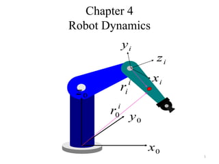
1. Chapter 4
Robot Dynamics
i
ir ix
iy
iz
0x
0z
0y
i
r0
1

2. Joint Velocity / Link velocity
• The velocity of a point along a robot’s link can be
defined by differentiating the position equation of the
point, which is expressed by a frame relative to the
robot’s base, .
• Here, we will use the D-H transformation matrices ,
to find the velocity terms for points along the robot’s
links.
(1)
• For a six-axis robot, this equation can be written as
(2)
P
R
T
iA
AAAATTTTT n321n
1n
3
2
2
1
1
R
H
R
...... 

AAAATTTTT 63216
5
3
2
2
1
1
0
6
0
...... 
2

3. Velocity of a link or joint
• Referring to equation on lecture 11b slide #9, we see
that the derivative of an matrix for revolute joint with
respect to its joint variable is
(3)
i
iA


















1000
dCS0
SaSCCCS
CaSSCSC
iii
iiiiiii
iiiiiii
ii
iA



















1000
0C00
CaSSCSC
SaSCCCS
i
iiiiiii
iiiiiii



3

4. Velocity of a link or joint
• However, this matrix can be broken into a constant
matrix and the matrix such that
(4)
(4)
iQ iA














1000
dCS0
SaSCCCS
CaSSCSC
X
iii
iiiiiii
iiiiiii


















1000
0C00
CaSSCSC
SaSCCCS
i
iiiiiii
iiiiiii














 
0000
0000
0001
0010
ii
i
i
AQ
A



 4

5. Velocity of a link or joint
• Similarly, the derivative of an matrix for a prismatic joint
with respect to its joint variable is
• which, as before, can be broken into a constant matrix and
the matrix such that
iQ
iA












0000
1000
0000
0000




















1000
dCS0
SaSCCCS
CaSSCSC
dd iii
iiiiiii
iiiiiii
ii
iA



(6)
iA













0000
1000
0000
0000












0000
1000
0000
0000














1000
dCS0
SaSCCCS
CaSSCSC
x
iii
iiiiiii
iiiiiii



(7)
5

6. Velocity of a link or joint
• In both equations (4) and (8), the matrices are always
constant as shown and can be summarized as follows:
iQ













0000
1000
0000
0000
prismaticQi )(
(8)
(9)
ii
i
i
AQ
d
A



,)(











 

0000
0000
0001
0010
revoluteQi
6

7. Velocity of a link or joint
• Using , to represent the joint variables ( for
revolute joints and for prismatic joints), and
extending the same differentiation principle to the
matrix of equation (2) with multiple joint variables (
and ), differentiated with respect to only one
variable gives
• Since is differentiated only with respect to one variable
, there is only one .
• Higher order derivatives can be formulated similarly from
iq
(10)
,..., 21 
,..., 21 dd
s'
sd'
iq
,21
21
0
....
)....(
ijj
j
ij
j
i
ij AAQAA
q
AAAA
q
T
U 





 ij 
i
0
T
jq jQ
k
ij
ijk
q
U
U



(11)
7

8. Velocity of a link or joint
• Using , to represent a point on link i of the robot
relative to frame i we can express the position of the
point by premultiplying the vector with the
transformation matrix representing its frame:
ir
(12)
(13)
i
ir ix
iy
iz
0x
0z
0y
ip
ii
0
ii
R
i rTrTp 
Same point w.r.t the base frame













1
z
y
x
r
i
i
i
i
A point fixed in link i and expressed w.r.t. the i-th
frame 8

9. Velocity of a link or joint
• Therefore, differentiating equation (12) with respect
to all the joint variables yields the velocity of the
point:
(14)
jq
 




i
1j
ijiji
i
1j
j
j
i
0
ii
0
i rqUrq
q
T
rT
dt
d
V )()()( 
The effect of the motion of joint j on all the points on link i
9

10. Velocity of a link or joint
Example 4.4
• Find the expression for the derivative of the
transformation of the fifth link of the Stanford Arm
relative to the base frame with respect to the second and
third joint variables.
 Solution
• The Stanford Arm is a spherical robot, where the second
joint is revolute and the third joint is prismatic.
• Thus,
543215
0
AAAAAT 
543221
2
5
0
52 AAAAQA
T
U 



 10

11. Velocity of a link or joint
where and are defined in equation (9).
 Example 4.4
• Find an expression for of the Sanford Arm.
 Solution
6543216
0
AAAAAAT 
543321
3
5
0
53 AAAQAA
d
T
U 



2Q 3Q
635U
6543321
3
6
0
63 AAAAQAA
d
T
U 



65543321
5
63
0
635 AAQAAQAA
q
T
U 



11

12. 12
Velocity of a link or joint
X0
Y0
X1
Y1
1
L
m













1
0
0
l
r1
Example: One joint arm with point mass (m)
concentrated at the end of the arm, link length is
l , find the dynamic model of the robot using L-E
method.
Set up coordinate frame as in the figure
]0,0,8.9,0[ g
1
11
11
11
0
1 r
1000
0100
00CS
00SC
rTp











 




13. 13
Velocity of a link or joint
X0
Y0
X1
Y1
1
L
m
1
1
1
111
0
111
0
11
0
0
Cl
Sl
qrTQrT
dt
d
pV 


















..

14. KINETIC ENERGY
AND
POTENTIAL
ENERGY
14

15. Kinetic and potential energy
 Kinetic Energy
• As you remember from your dynamics course, the kinetic
energy of rigid body with motion in three dimensions is
(Fig.1 (a))
where is the angular momentum of the body about G.
G
2
h
2
1
Vm
2
1
K .
Gh
G
(a)


V
G
(b)
Fig. 1 A rigid body in three-dimensional motion and in plane
motion
(1)
15

16. Kinetic and potential energy
• The kinetic energy of rigid body in planar motion (Fig. 1
(b))
• The kinetic energy of the element of mass on link is
• Since has three components of it can be
written as matrix, and thus
.22
I
2
1
Vm
2
1
K 
im
dmzyx
2
1
dK
2
i
2
i
2
ii )(
...

(2)
(3)
iV ,,,
..
iii zyx














2
iiiii
ii
2
iii
iiii
2
i
zyzxz
zyyxy
zxyxx
.....
.....
.....


















 iii
i
i
i
T
ii zyx
z
y
x
VV
...
.
.
.
(4)
16

17. Kinetic and potential energy
and
• Combining equations (14) and (3) yields the following
equation for the kinetic of the element:
where p and r represent the different joint numbers.
• This allows us to add the contributions made to the final
velocity of a point on any link I from other joints
movements.
2
i
2
i
2
i zyx
...

(4)
(6)













2
iiiii
ii
2
iii
iiii
2
i
T
ii
zyzxz
zyyxy
zxyxx
TraceVVTrace
.....
.....
.....
)(
,])).()(.)([(
.
i
T
i
i
1r
r
iri
i
1p
p
ipi dmr
dt
dq
Ur
dt
dq
UTrace
2
1
dK  

17

18. Kinetic and potential energy






    
i
1p
rp
T
ir
T
iiip
i
1r
ii qqUdmrrUTr
2
1
dKK )(




































 




iiiiiii
ii
zzyyxx
yzxz
iiyz
zzyyxx
xy
iixzxy
zzyyxx
iii
i
2
iiiii
iii
2
iii
iiiii
2
i
T
iii
mzmymxm
zm
2
III
II
ymI
2
III
I
xmII
2
III
dmdmzdmydmx
dmzdmzdmzydmzx
dmydmzydmydmyx
dmxdmzxdmyxdmx
dmrrJ













1
z
y
x
r
i
i
i
i
Center of mass
 dmx
m
x i
i
i
1
Pseudo-inertia
matrix of link i
•Integrating equation (6) and rearranging terms yields the total kinetic
energy:
(7)
(8)
18

19. Kinetic and potential energy






   
n
1i
rp
T
iriip
i
1r
i
1p
i qqUJUTr
2
1
K )(
•Substituting equation (8) into equation (7) gives the form
for kinetic energy of the robot manipulator:
•The kinetic energy of the actuators can also be added to
this equation.
•Assuming that each actuator has an inertia of , the
kinetic energy of the actuator is , and the total
kinetic energy of the robot is
(9)
(10)
)(actiI
2
iacti qI21
.
)(/
   







n
1i
2
iacti
n
1i
rp
T
iriip
i
1r
i
1p
i qI
2
1
qqUJUTr
2
1
K
.
)()( 
19

20. Kinetic and potential energy
)]([ ii
0T
i
n
1i
n
1i
i rTgmPP   
Potential Energy
•The potential energy of the system is the sum of the
potential energies of each link and can be written as
where is the gravity matrix and is
the location of the centre of mass of a link relative to the
frame representing the link.
matrix and position vector
matrix.
(11)
],,,[ oggggT
 ir
4X1gT

1X4rT ii
0

20

21. 21
Motion Equation of
a
Robot Manipulator

22. Motion equations of a robot manipulator
 The Lagrangian can now be differentiated in order to form
the dynamic equations of motion.
 The final equations of the motion for a general multi- axis
robot can be summarized as follows:
(1)
(2)
(3)
(4)
22

23. Motion equations of a robot manipulator
 In Equation (1), the first part is the angular acceleration-
inertia terms, the second part is the actuator inertia term,
the third part is the Coriolis and centrifugal terms and the
last part is the gravity terms.
 This equation can be expanded for a six-axis revolute
robot as follows:
(4)
23

24. Motion equations of a robot manipulator
 Notice that in equation (4) there are two terms with .
 The two coefficients are and .
 To see what these terms look like, let’s calculate them for
i=4.
 Form equation (3), for , we will have i = 4, j = 1, k =
2, n= 6, p = 4 and for , we have i = 4, j = 2, k= 1, n =
6, p = 4, resulting in
(6)
21
21iD 12iD
512D
521D
24

25. Motion equations of a robot manipulator
and from equation (6) we have
(7)
25

26. Motion equations of a robot manipulator
• In these equations, are the same.
• The indices are only used to clarify the relationship with
the derivatives.
• Substituting the result from equation (7) into (6) show that
• Clearly, the summation of the two similar terms yields the
corresponding Coriolis acceleration term for .
• This is true for all similar coefficient in equation (4).
• Thus, we can simplify this equation for all joints as
follows:
(7)
21andQQ
521512 UU 
21
26

27. Motion equations of a robot manipulator
(8)
(9)
27

28. Motion equations of a robot manipulator
(10)
(11)
28

29. Motion equations of a robot manipulator
(12)
(13)
29

30. Motion equations of a robot manipulator
30

31. Motion equations of a robot manipulator
Example
Using the aforementioned equations, derive the equations of
the motion for the two-degree-of-freedom robot arm. The
two links are assumed to be of equal length.
31

32. Motion equations of a robot manipulator
Solution
To use the equations of motion for the robot, we will first
write the A matrices for the two links; the we will develop
the terms for the robot.
Finally, we substitute the result into equations (8) and (9) to
get the final equation of the motion.
The joint and the link parameters of the robot are
iijkij DandDD ,,,
00lala0d0d 212121   ,,,,,
32

33. Motion equations of a robot manipulator
33

34. Motion equations of a robot manipulator
34

35. Motion equations of a robot manipulator
35

36. Motion equations of a robot manipulator
From equation (8), assuming that products of inertia are
zero, we have
36

37. Motion equations of a robot manipulator
For a two-degree-of-freedom robot, robot, we get
From equation (2), (3), and (4) we have
(14)
(14)
37

38. Motion equations of a robot manipulator
38

39. Motion equations of a robot manipulator
ll
39

40. Motion equations of a robot manipulator
Substituting the results into equations (14) and (14) gives
the final equations of motion, which, except for the
actuator inertia terms, are the same as equations (7) and
(8) of L-E formulation.
40