Retrospective Theses and Dissertations
Iowa State University Capstones, Theses and
Dissertations
1959
Relation of fertilization rates to pasture yield and
utilization
William Owen McCarthy
Iowa State University
Follow this and additional works at: https://lib.dr.iastate.edu/rtd
Part of the Agricultural and Resource Economics Commons, and the Agricultural Economics
Commons
This Dissertation is brought to you for free and open access by the Iowa State University Capstones, Theses and Dissertations at Iowa State University
Digital Repository. It has been accepted for inclusion in Retrospective Theses and Dissertations by an authorized administrator of Iowa State University
Digital Repository. For more information, please contact digirep@iastate.edu.
Recommended Citation
McCarthy, William Owen, "Relation of fertilization rates to pasture yield and utilization " (1959). Retrospective Theses and Dissertations.
2135.
https://lib.dr.iastate.edu/rtd/2135

RELATION OF FERTILIZATION RATES
TO PASTURE YIELD AND UTILIZATION
by
William Owen McCarthy
A Dissertation Submitted to the
Graduate Faculty in Partial Fulfillment of
The Requirements for the Degree of
DOCTOR OF PHILOSOPHY
Major Subject: Agricultural Economics
Approved:
In Charge of Major Work
Head of Major Departme:
Iowa State College
Ames, Iowa
1959
Signature was redacted for privacy.

il
TABLE OF CONTENTS
Page
I. INTRODUCTION 1
II. OBJECTIVES 5
III. SOURCE OF BASIC DATA 7
IV. DERIVATION OF PRODUCTION FUNCTIONS 8
V. DERIVATION OF ECONOMIC OPTIMA 32
VI. NUMBER OF CUTTINGS UNCERTAIN 58
VII. THE UTILIZATION PROBLEM 78
VIII. UTILIZATION AND NUMBER OF CUTTINGS UNCERTAIN . 88
IX. SUMMARY AND CONCLUSIONS 104
X. BIBLIOGRAPHY . . '. , 108
XI. ACKNOWLEDGEMENTS 110
XII. APPENDIX A. MIDMONTH PRICES RECEIVED BY
IOWA FARMERS FOR ALFALFA HAY AT
LOCAL MARKETS Hie
XIII. APPENDIX B. PROCEDURE FOR VALUING ALFALFA
FED GREEN CHOPPED TO DAIRY COWS 112
XIV. APPENDIX C. PROCEDURE FOR VALUING ALFALFA
PASTURE FED TO PIGS 115

1
I. INTRODUCTION
A. General
One central problem confronts any farmer acting in his
capacity as a decision maker. It concerns planning for a
future which is always uncertain in respect to yields, prices,
or both. A drought may parch his land to an extent that in
one year his crops are scarcely worth harvesting. In another
year seeds or young plants may be washed out by excessive rain
or floods. Yet, in another growing season, climatic factors
may combine favorably to provide him with bumper crops. Added
to this, the free market mechanism usually penalizes him in
price when he and his neighbors have a large crop or livestock
output. In contrast, in years of drought, his small output
does not allow him to take advantage of high prices.
In practice the conditions that the farmer faces may not
be as extreme as those suggested. The examples, however,
emphasize that ex ante manipulation of resources in order to
maximize future value product, presents decision making prob
lems •
Consider decisions centering around fertilizer use• The
decision of whether or not to use fertilizer might seem easy
under today's scientific farming methods. Yet in 1954 only
58 percent of Iowa farmers used fertilizer. The average
amount spread was only 5.5 tons per farm (21).

2
However, once It has been decided to use fertilizer, a
whole new series of choices must be made. Ideally, a choice
of specific fertilizer elements should be made on the basis
of soil test data and known crop requirements. But often the
former are not available for the individual farm. Thus in
using an NPK fertilizer mix, as opposed to NP or PK mixtures,
the farmer may be motivated by personal preference or the
theory that a little of everything is beneficial. Altern
atively the neighbors or the fertilizer salesman may influ
ence him. The rate of application per acre may depend on such
factors as the mechanical condition of the manure distributor
i
or the expected crop or pasture yield. Or the deciding in
fluence may be advice of farmer friends or extension workers.
This study seeks to demonstrate that some precision can
be given to decisions concerning fertilizer use, even in the
presence of uncertainty. Particular attention is paid to only
a few of the factors that the farmer takes into account.
Hence the analysis may possibly be criticized on the grounds
of over simplification.
Initially the farmer decision maker is considered to be
concerned only with the problem of the profit maximizing rate
of fertilization of alfalfa, when one, two or three cuttings
can be expected with certainty. Different capital situations
are examined. The amount of money available for buying fer
tilizer may or may not be limited. The farmer may or may not

3
apply fertilizer, depending on how he considers the returns
compare, if the money was spent on other Inputs.
The second more realistic case assumes that the farmer
is uncertain as to whether he will get one, two or three cuts
from his alfalfa.
The various optima are all arrived at as if they were
ex post decisions. Unhappily, as every extension worker
knows, the farmer requires ex ante advice. Few advisory
workers would be willing to base predictions on the result of
one experiment carried out under particular environmental con
ditions. However they would probably admit that the data
would have predictive value for future experiments, if the
circumstances surrounding these later experiments were sim
ilar. A series of trials on different soil types and in dif
ferent locations would enable reliable recommendations to be
made. These are the grounds for asserting that advice based
on ex post information can help to reduce decision making
uncertainty.
There is another aspect of fertilizer use. The quantity
of fertilizer applied may be based not only on expected yields
but also on the method of utilization of the crop. The far
mer may sell alfalfa as hay rather than keep it for feeding
purposes. If the hay is sold he may be prepared to apply a
greater quantity of fertilizer, in expectation of higher

4
profits.
Therefore the third case deals with an extension of the
first (in which yield is certain). In addition it is assumed
that utilization is certain. The alfalfa may be kept as hay
for winter supplementary feed or it may be sold. Alternative
ly it may be used greenchopped for dairy cows or as summer
pasture for pigs.
Throughout the growing season the value of the alfalfa
in various uses may change. Thus a drought may force the far
mer to feed in situ rather than as hay. Acquisition of labor
saving machinery may reduce the cost of haymaking. This leads
to the fourth case to be examined. This is essentially a
yield uncertainty situation. In addition, there is uncer
tainty concerning the utilization of the crop, at the time
of application of the fertilizer.
The analysis is relatively simplified as compared to the
onfarm situation. But it does reduce some of the variable
elements in decision making to more measurable terms.

5
II. OBJECTIVES
The previous chapter gave a general review of the area
in which the study is being made.
More specifically, the objectives are: (a) to decide on
the form of a production function which best expresses the
relationship between PgOg and KgO application and alfalfa
yield for a particular experiment; (b) to fit this function
to the yield data from the experiment; (c) to attempt to de
rive profit maximizing fertilization rates for the alfalfa
under specific circumstances. These circumstances relate to
the number of cuttings and the method of utilization of the
crop.
The first two aims are discussed in Chapter IV. The
third objective is the major preoccupation of the study.
Chapter V examines the situation in which the number of cut
tings is certain. Capital available for fertilizer is first
considered unlimited, then later assumed restricted. In
Chapter VI profit maximization is discussed when the number
of cuttings expected is uncertain. Chapter VII considers
that utilization of the crop is known ex ante. It is shown
that fertilization levels may be adjusted accordingly. In
Chapter VIII both utilization and the number of cuttings are
assumed unknown when the fertilizer is applied. Alternative
fertilizer use decisions are examined for this situation.

6
In general the aim of the analysis is to show that pre
cision can be given to fertilizer use recommendations

7
III. SOURCE OF BASIC DATA
The experiment from which the data were obtained was one
of a series of pasture fertilization trials. These were car
ried out in southeast Iowa under the direction of the Agronomy
Department of Iowa State College. The trial analyzed in this
study was laid down on Weller silt loam in Van Buren County
in 1952. The design was a 3 x 3 factorial, replicated twice,
giving a total of 18 observations. Two of these were checks.
PgOg and KgO fertilizer were both applied at three levels
(0, 60 and 120 pounds per acre). The alfalfa was cut three
times during the course of the growing season. Three cuttings
are considered normal in this area. Table 1 includes the re
sults of these three cuttings.
Table 1. Weller silt loam, yields of alfalfa, 1952 (tons
oven dry material per acre)
Rate of fertilization 1st cut 2nd cut 3rd cut
(lbs./acre) Replicate Replicate Replicate
p2°5 Kg° I II I II I II
0 0 .73 .84 .69 .95 .45 .55
60 0 .94 1.41 .85 .95 .60 .50
120 0 1.16 1.38 .83 .92 .62 .57
0 60 1.05 1.21 .85 .85 .55 .57
60 60 1.32 1.49 .92 .92 .65 .67
120 60 1.27 1.56 .97 1.16 .62 .72
0 120 1.05 1.32 .90 .92 .57 .62
60 120 1.49 1.27 1.00 1.00 .69 .57
120 120 1.68 1.38 1.07 1.00 .67 .65

8
IV. DERIVATION OF PRODUCTION FUNCTIONS
A. Introduction
Chapters I, II and III outlined the scope and nature of
the study. The basic yield data around which the analysis is
built were also presented. This chapter discusses the altern
ative forms of production functions which might be used. Re
gression equations are then presented, together with their
consequent statistical tests of significance. Finally, pro
duction surfaces, 1soquants and isoclines are shown and dis
cussed.
B. Selection of a Function
There is agreement in the literature on fertilizer pro
duction functions (9, 14) about the form of function to be
chosen as best representing the relationship between input
and output quantities. It should be some compromise between
what is biologically compatible and what is statistically
sound. Less emphasis has been placed on the ease and reli
ability with which economically meaningful quantities can be
derived from the function. A practical consideration which
must be taken into account is that time and research funds
are not limitless. This is true for researchers working in
a nonacademic environment and for some university personnel.
It may be desirable for work to be pressed forward in seeking

9
an "ideal" function characterizing response of plants to
fertilizer. However, the fact remains that guidance must be
given now to farmers end others.
Fortunately the choice of a suitable form of function is
not as difficult as it might appear. The more generally
acceptable^ types of functions fall into three groups: (a)
exponentials, (b) the power function (CobbDouglas) and (c)
polynomials.
The most widely used exponentials are the Mitscherlich
and the Spillman. But these lack elegance from the computa
tional point of view. Also they have the disadvantage that
statistical tests such as standard errors and t values cannot
be computed, for the coefficients. Again the product curve
for both is regarded as asymptotic to some maximum yield.
This fact is not easily reconcilable with observed phenomena
of negative marginal products found in some fertilizer experi
ments. The assumption that elasticity of response is less
than 1 over all ranges of inputs may not be realistic at the
lower rates of fertilization. This is especially true for an
impoverished soil.
The power function presents no computational problems
and is amenable to statistical tests. But the assumption of
•'•Ruling out such special cases as the Bray modification
of the Mitscherlich, Janisch's complex exponential, or Briggs1
hyperbolic form.

10
constant elasticity of production may be justifiable only for
a small range of fertilizer inputs. Relaxation of the
assumptions of constant elasticity and symmetry gives a more
realistic form (6). Unfortunately the computations for find
ing economic optima become extensive.
By contrast, polynomial models are easy to fit and test.
Also they are flexible in the sense that terms may be added
or dropped easily. Furthermore, no assumptions are made about
the. elasticity of response. Negative marginal products are
allowed for by the inclusion of a squared term with (usually)
negative sign. (The signs do not always work out to be nega
tive, in which case the problem of adjusting for diminishing
returns remains unsolved.) The chief criticism of such func
tions is that only linear and interaction terms can be justi
fied as far as plant growth is concerned. The same cannot be
said for squared or cubed terms or terms raised to some oower
(e.g.. square root transformations). Thus inconsistencies of
one sort or another can be found in all these functions seek
ing toqquantify inputoutput relationships. Eventually a
choice, not based entirely on objective grounds must be made.
As far as the present study is concerned, a polynomial
function with an interaction term Was used. Specifically,
the form of function is as follows:
Y = a + bP + cK dP^ eK+ fPH where
Y = expected yield; a = yield Intercept; b, c, d and e are

11
the regression coefficients and P and K are the fertilizer
inputs.
It was decided to fit a quadratic rather than a square
root function. This is in accord with the criteria used by
Heady (8) in selecting between these two types of polynomials.
The alfalfa yields of Table 1 provide the basic data
used in this study. As a foundation for the analysis which
follows a regression equation has been fitted to the data of
each cutting. Yields for the first and second cuttings were
added together and a further function was fitted to this
total. Likewise a regression equation wss computed for the
sum of the yields of the three cuttings.^ The five equations
presented in the order mentioned above are:
Y = .822235 + .007042P + .00618IK .000028P2
C. Regression Analysis
.000027K2 .000010PK
Y = .811947 + .001278P + .001403K .000004P2
.000006K2 + .000005PK
(4.1)
(4.2)
Y = .490277 + .001431P + .00218IK .000005P
.000012K2 .000002PK (4.3)
^Subsequent interpretation of the data in terms of hay
rather than oven dry material means that the regression co
efficients alter slightly.

12
Y = 1.634182 + .008320P + .007584K .000032P2
.000033K2 .000005PK (4.4)
Y = 2.124459 + .009751P + .009765K .000037P2
.000045K2 .000007PK (4.5)
Equation 4.4 could have been obtained by adding 4.1 and 4.2
and equation 4.5 by aiding 4.1, 4.2 and 4.3. However as a
further check on accuracy separate regressions were computed.
Table 2 includes the analyses of variance for the yield
data corresponding to each of the above regression equations.
In assessing whether the function chosen characterizes the
data adequately, one common criterion is the size of the
P 1
R s . In Table 2 these seem satisfactory when compared with
the R2's derived from similar data (3, 10).
The overall significance of the regressions were tested
by means of the F ratio (the null hypothesis is b'y^ = b'y^
etc• =0). Of the data of most interest in future chapters,
namely the first cut, the first plus second cut and the
first plus second plus third cut, the F's are all significant
at less than the 5 per cent level. For the second and third
cuts taken by themselves, the F values fall Just outside the
5 per cent level.
A further criterion suggested by Mason (14) Is that the
1r2 _ Reduction in sum of squares due to regression
Treatment sum of squares

Table 2 - Weller silt loam, analyses of variance for alfalfa cuttings
Source of variation
Degrees
of
freedom
Sum of
squares
Mean
square
Cutting 1
(Regression 4.1)
R2 = .959
R = .979
Total
Replicates
Treatments
Due to regression 5
Lack of fit 3
Error
17
1
8
8
.743363
.031348
1.090361
.076049
.774711
.148672 4.96*
.239601 .029950
Cutting 2
(Regression 4.2)
R2 = .863
R = .929
Total
Replicates
Treatments
Due to regression 5
Lack of fit 3
Error
17
1
8
8
.098539
.015605
,177694
.019338
.114144
.019708 3.57+
,044212 .005526
«
Cutting 3
(Regression 4.3)
R2 = .918
R = .958
Total
Replicates
Treatments
Due to regression 5
Lack of fit 3
Error
17
1
8
8
.049753
.004458
,079511
0
.054211
,025300
.009951 3.IS1
.003162
*P <.05
+P ===.05

Table 2. (Continued)
Degrees
of Sum of Mean
Source of variation freedom squares square F
Cuttings 1+2
(Regression 4.4)
R2 = .982
R = .991
Total
Replicates
Treatments
Due to regression
Lack of fit
Error
5
3
17
1
8
8
1.353403
.025097
1.434600
.172088
1.378500
.270681 5.04*
.384012 .048001
Cuttings 1+2+3 Total
Replicates
Treatments
r" = .979 Due to regression
R = .989 Lack of fit
Error
5
3
17
1
8
8
1.911847
.041197
2.601844
.172088
1.953044
.382369 6.42**
.476712 .059589
**P *=.01

15
lack of fit term should be of the same order of magnitude (or
less) than the experimental error. In the cases under con
sideration, the lack of fit terms are considerably less than
the error terms.
On the basis of these tests it is assumed that the
quadratic function characterizes the data adequately.
Whether or not individual terms should be dropped from
the equations can be solved statistically by computing the t
values and the standard errors of each coefficient. Table 3
includes these values for the equations. If terms are to be
dropped on the basis of the t test alone and assuming that
the 5 per cent level of significance is the critical one,
P p
then a number of terms would be discarded. These are P , K
and PK from 4.1 and 4.4 and P2 and PK from 4.5.
A more lenient criterion is proposed by Anderson (1).
A variable is dropped only if the standard error of the re
gression coefficient exceeds the estimated coefficient. As
far as equations 4.1, 4.4 and 4.5 are concerned this means
that only the PK term would be dropped in each case.
In practice other considerations affect the final form
? P
of the equation. If the P and K terms are dropped from
equation 4.1 this assumes linear response of alfalfa growth
to all levels of Pg05 and KgO fertilization. Inclusion of a
squared term is not easy to interpret individually where
plant growth is concerned. But as far as the whole equation

Table 3. Standard errors and t values for equations 4.1 to 4.5
P K p2 K2 PK
Equation 4.1 .007042 .006181 .000028 .000027 .000010
Standard errors .002865 .002723 .000020 .000019 .000015
t values
sa
2.59 2
.27 1.36 1.29 .67
Probability levels of t'sa .01 .05 .20 .20 .50
Equation 4.2 .001278 .001403 .000004 .000006 .000005
Standard errors .002028 .002033 .000015 .000015 .000011
t values .63 .69 .26 .39 .45
Equation 4.3 .001431 .002181 .000005 .000012 .000002
Standard errors .001044 .001048 .000008 .000008 .000005
t values 1.87 2
.08 .58 1.46 .37
Equation 4.4 .008320 .007584 .000032 .000033 .000005
Standard errors .002432 .002430 .000018 .000019 .000013
t values
sa
3.42 3.12 1.73 1.77 .37
Equation 4.5 .009751 .009765 .000037 .000065 .000007
Standard errors .003038 .003033 .000023 .000023 .000016
t values 3.21 3.22 1.59 1.92 .43
^Probability of drawing s. t value as large or larger given the null hypothesis.

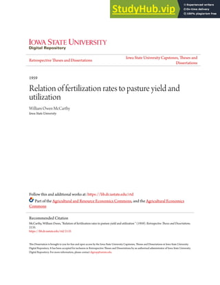
17
goes, it does permit diminishing returns. Thus the equation
gives a picture of plant growth more in keeping with accepted
theory. Hence squared terms have been retained.
The inclusion of a PK term is easier to Justify on bio
logical grounds. Some interaction between PgOg and KgO might
be expected which would have an influence on plant growth.
Thus in spite of the fact that the t's and the standard
errors for all the PK's are low, it was decided to retain
this term in the equations.
D. Nature of the Production Surfaces
Regression equations 4.1, 4.4 and 4.5 were used to de
rive expected yields of alfalfa for various Pg0$ and KgO
levels. These are shown in Table 4. The data from this
table has been used to construct the production surfaces of
Figures 1, 2, 3 and 4.
Figure 1 shows the nature of the production surface
obtained when yields from the first cutting of alfalfa are
considered alone. The relevant range of fertilization for
the experiment was from 0120 pounds per acre, for both
nutrients. But it was felt that for illustrative purposes
extrapolation beyond this range was Justified. This was be
cause of the goodness of fit of the regressions and because
of the symmetrical nature of the estimating equations.
Figure 1 indicates that with KgO held constant at some

18
Table 4. Expected yields of alfalfa (tons oven dry material
per acre) for various PgOg and KgO levels (lbs.
per acre)
K
P 0 40 80 120 160 . 200
1st cut 0 .822 1.026 1.143 1.175 1.120 .978
40 1.059 1.267 1.348 1.364 1.293 1.135
80 1.206 1.378 1.463 1.463 1.376 1.202
120 1.264 1.620 1.489 1.473 1.370 1.180
160 1.232 1.372 1.425 1.393 1.274 1.068
200 1.110 1.234 1.271 1.223 1.088 .866
1st + 2nd 0 1.634 1.884 2.030 2.069 2.002 1.831
cut 40 1.916 2.158 2.296 2.327 2.252 2.073
80 2.095 2.329 2.459 2.482 2.399 2.212
120 2.171 2.397 2.519 2.534 2.443 2.248
160 2.146 2.364 2.478 2.485 2.386 2.183
200 2.018 2.228 2.334 2.333 2.226 2.015
1st + 2nd 0 2.124 2.443 2.617 2.048 2.534 2.277
4 3rd 40 2.655 2.763 2.926 2.945 2.820 2.552
cut 80 2.667 2.964 3.115 3.124 2.987 2.708
120 2.761 3.046 3.187 3.184 3.037 2.746
160 2.737 3.011 3.140 3.127 2.968 2.666
200 2.594 2.857 2.975 2.950 2.780 2.467
level, as the amount of PgOg fertilizer applied per acre
grows heavier the yield of alfalfa increases. The maximum
yield is obtained et a PgOg level of 120 pounds. Thereafter
addition of further quantities of PgOg cannot check the de
crease in total yield. On the other hand, for low levels of
PgOg, the maximum yield of alfalfa is obtained when the
amount of KgO required decreases. Thus when PgOg is applied
at the rate of 200 pounds per acre, only 80 pounds of KgO

19
2000
1750
LU
CXL
O
<
£1500
£L
CL
LU
H 1250
<
1000
>
ex.
Q
CO
z
Q
I
û 750
_i
UJ
>
< 500
_i
S
250
200
,60^
120 ^
, * 0
Les
e o o * *
Figure 1. Production surface for 1st cutting of alfalfa

20
3000r
2750
LU
o2500
<
S 2250 "
QL
UJ
|Z 2000
<
£ 1750
o
i
f
)
z 1500
g
o 1250
_J
UJ
v 1000
<
u_
g 750
Figure 2. Production surface for lst+Pnd cuttings of alfalfa

21
3250
3000
2750
LU
(K
< 2500
a
:
LU
o. 2250
û:
LU
h 2000
<
£ 1750
o
V)
z
o
h
500
o 1250
_i
UJ
>
<
LL
_J
2
<
000
750
500
250
0
Z
H'"te!0
4cëe 2°o
Figure 3. Production surface for lst+?nd+3rd cuttings
of alfalfa

22
are necessary to maximize yield.
Figure 2 illustrates the shape of the surface obtained
when alfalfa yields from the first and second cuttings are
aggregated. As the level of PgO§ is increased, while holding
KgO constant, there Is a sharp yield response. Yield reaches
its maximum when the quantity of PgOç is approximately 120
pounds per acre (irrespective of the KgO level). Contrari
wise, when PgOg remains constant, and the amount of KgO is
increased, the highest alfalfa yields occur initially when
KgO is at 120 pounds per acre. But as the PgOg level in
creases, the amount of KgO necessary for attainment of a max
imum yield decreases to 80 pounds. Thus as in Figure 1
(under similar circumstances) the relationship is one of
nutrient substitutability.
The production surface Illustrated in Figure 3 is the
one corresponding to the total alfalfa yield for the whole
season (first plus second plus third cuttings). When KgO
is held constant and PgO§ is increased, then, as in the two
previous cases, the maximum alfalfa yield is obtained when
Pg05 is applied at 120 pounds per acre. But Pp05 may be
held at various levels and KgO increased. Then for all
levels of PgO5 an application of 100 pounds per acre of KgO
gives a maximum alfalfa yield.
Figure 4 brings Figures 1, 2 and 3 together for compara

uj 3250
CE
O
<3000
cc
^2750
52500
<2250
>2000
z
g 1500
o 1250
LU
£ 1000
L? 750
_i
<
uï 500
250
0 Hias°>
&)
40 o ^
+

<
i
-
' £
°
/
o
°
o ^
ro
OJ
"s
l
e
t^0
0
Figure 4. Production surfaces for 1st, lst+gnd and lst+2nd+3rd cuttings
of alfalfa

24
tive purposes. A noticeable feature of the diagram is that
the three surfaces are all good examples of the classical
increasingdecreasing total returns pattern. The compara
tive heights of each surface are a. reflection of the total
yield after each cutting. The differences in heights repre
sent the addition to total yield due to the extra cutting.
The second cutting was heavier than the third (as is reflected
in equations 4.2 and 4.3). Hence the increase in height of
the second surface from the first is greater than the increase
from the second to the third.
E. Nature of the Yield Isoquants
Isoquants were derived from the basic production func
tions 4.1, 4.4 and 4.5 by assuming values for one nutrient
and yield (Y) and solving for the other nutrient. Isoquant
equations for the first cutting (4.6), the first plus second
cuttings (4.7) and the first plus second plus third cuttings
(4.8) are shown on page 25.
Equations 4.6, 4.7 and 4.8 were used to derive the iso
quants shown in Figure 5. A set of three isoquants are shown
for eacn equation. The isoquants predict various combinations
of P2O5 and KgO required to produce a particular alfalfa
yield. Some of these combinations ^re shown in Table 5.
Thus for one cutting, 5 pounds of KgO and 35 pounds of P<?05
or 25 pounds of KgO and 7 pounds of PgOg give a yield of 1.2

es
( .007887.000011K) + /(.007887.000011K)24(.000031)(Y.006923K+
.00006?
(•009318.000006K) + .009318.000006K)?4( .000036)(Y.0C8494B
•00007?
(.010991.000008K) + /(.0109P1.000009K)?4( .000041)(Y.010937K
.00008?

J23K+.000030K?.920903
(4.6)
3494K+.000037K21.830284
(4i7)
)937K+.000050K22.379394
(4.8)

26
80
A = 1st CUTTING
B 1st + 2nd CUTTINGS
C= 1st + 2nd + 3rd CUTTINGS
70
60
40
30
20
q
0 10 20 30 40 50 60
K20, POUNDS PER ACRE
Figure 5. Isoquants for 1st, lst+?nd end lst+Pnd+3rd
cuttings of plfslfs hey

27
Table 5. Fertilizer combinations and corresponding marginal
rates of substitution for various hay yields
MRS& MRSa MRS®
Lb. Lb. P205 Lb. P2O5 Lb. P9O5
KgO ?20|
5 for KgO KgO p2°£i for KgO KgO Pp05 for KgO
1st cut 1st cut 1st cut
1.2 tons per acre 1.3 tons per acre 1.4 tons per acre
5 35 .908 5 54 .744 5 84 .460
10 27 1.013 10 45 .856 10 69 .629
20 13 1.230 20 28 1.095 20 49 .893
25 7 1.343 30 14 1.346 30 31 1.178
30 0 1.475 40 0 1.656 50 2 1.849
lst+2nd cut lst+2nd cut lst+2nd cut
5 37 .838 5 53 .701 5 75 .507
10 26 .972 10 41 .840 10 59 .677
15 16 1.108 15 30 .981 20 37 .962
20 8 1.238 20 20 1.125 30 15 1.303
25 0 1.380 25 11 1.273 35 6 1.479
lst+2nd+3rd cut lst+2nd+3rd cut lst+2nd+3rd cut
b 38 .766 5 69 .528 10 108 .219
10 30 .864 10 59 .634 20 79 .516
15 22 .971 20 40 .868 30 49 .883
20 15 1.079 30 23 1.134 40 30 1.216
30 2 1.328 40 9 1.437 50 17 1.573
aPounds of KgO replaced by 1 pound of P 5 O 5 .
tons of hay,
The isoquants are curved just enough to indicate dimin
ishing marginal rates of substitution. The change in slope
from left to right is gradual, indicating that the nutrients

28
are good substitutes, within the range of the experiment.
This is true for each set of isoquants.
Table 5 also includes marginal rates of substitution of
Pg05 for KgO. The marginal rate of substitution may be de
fined as the ratio of the marginal products of the two inputs.
The rates of substitution were derived from the left hand
sides of equations 4.9, 4.10 and 4.11 by substituting values
of KgO and PgO^+intb the equations. The marginal rate of
substitution indicates the change in the amount of one input
necessary to maintain a certain yield, when one unit of an
other input is added. In Table 5 the i soquant equation for
the 3.2 ton yield of the first plus second plus third cut
tings slopes sharply at its upper end. To maintain yield
1 pound of PgOg replaces a small amount of KgO. However as
the isoquant flattens out the amount of KgO replaced by each
pound of PgOtj becomes greater.
F. Nature of Yield Isoclines
Yield isoclines (least cost expansion paths) were de
rived by equating the marginal products of each production
function to the nutrient price ratio and solving for one
nutrient. Isoclines were worked out for the first, first
plus second, and first plus second plus third cuttings, so
tnat the relevant production functions were 4.1, 4.4 and 4.5.
The isocline equations corresponding to these functions are

29
presented below in the order mentioned. The nutrient price
ratio is represented by "a".
.00738? .000062P .OOOOllK „ (4.9)
.006923 .000060K .000011P
.009318 .000072P .000006K
.008494 .000074K .000006P
.010921 .000082P .000008K
= a
= a (4.10)
.01093? .000100K .000008P = & (4.11)
In Figure 6 an isocline family has been drawn for each
equation. Each isocline represents the least cost PgOg and
KgO combination for the nutrient price ratio shown. (The
actual PgOg and KgO prices are 10 cents and 5 cents per pound,
respectively, so that in reality pP/pK is P.O.) The relative
slopes of each set of isoclines do not differ greatly. As
an isocline is a line connecting all points of equal slope
on a family of isoquants it could be inferred that the slopes
of the corresponding sets of isoquants are also similar.
This is confirmed in Figure 5. The dotted lines are the
ridge lines (i.e., isoclines representing zero substitution
rates) beyond which the inputs will not substitute for each
o ther.
On any production surface where the yield attains a
maximum, the family of isoclines converge to a point. The
point is where the partial derivatives of both inputs are
zero. Maximum yields for the cuttings are predicted at sim
ilar fertilization rates. For one cutting alone, the amounts

30
Dashed lines are ridgelines
FOR 1st + 2nd CUT
—— Pp/P|< — 3.3
For 1st t 2nd + 3rd CUT
Pp/PK = 3.3
Pp/PK =2.0
Pp/PK = 1.4
FOR 1st CUT
tr 100
CL* 60
Figure 6,
40 60 80
K%0, POUNDS PER ACRE
Isoclines for 1st cut, lst+Pnd cut rnd
lst-t- 2nd+3rd cuts of Plfplf'? hay

31
of PgOc) and KgO required are smaller than for two or three
cuttings. To maximize yield for three cuttings more PgO$ but
less KgO is required tnan for two cuttings.
The first two objectives of this study have now been
attained. A function has been chosen and fitted. Statistical
tests have shown that it.characterizes the data adequately.
In addition, production surfaces, isoquants and isoclines
have been derived which conform to production function theory.
Chapter V will make use of the regression equations to derive
profit maximizing quantities of fertilizer.

32
V. DERIVATION OF ECONOMIC OPTIMA
A. Introduction
Due to past experience, there may be little uncertainty
in the farmers' mind as to the number of cuttings of alfalfa
expected. It is possible that he is not only subjectively
certain, but correct in his estimates. In any case he dis
criminates in use of fertilizer applied to alfalfa in the
early spring. The present chapter examines the profit max
imizing implications of vario us rates of fertilization.
The basic assumption is that the farmer has ex ante knowledge
of the number of cuttings expected.
Throughout the analysis it is necessary that a money
value be put on the hay crop, so that various optima may be
worked out. This value is taken as the local market sale
price. The justification for this approach is that should a
farmer wish to sell hay, its value is no greater than the
current market price. On the other hand he cannot impute a
higher than market value to his own hay. If he found that
his cost of production was higher than average, then, other
things being equal, he should buy, rather than make, hay.
Appendix A shows the range in prices received by Iowa farmers
for alfalfa hay for the period 19461958. Hay prices used
in subsequent computations are based on this range.
J'he discussion in this chapter is confined to four pos

33
sibilities. The first and simplest cp.se is the derivation
of profit maximizing quantities of fertilizer under the
assumption that the farmer has unlimited capital available
for its purchase. The second case is concerned with maxi
mization of returns per dollar invested in fertilizer. The
third possibility is that common fertilizer mixes are used
rather then specific quantities. The effect on profits of
using mixtures is shown. The fourth case centers around the
differences in net returns per dollar invested in fertilizer,
if mixtures are used. Finally graphs are presented to illus
trate the equating of marginal returns when fertilizer is
used for different crops. In working out profits due to
fertilization the only cost taken into account is that of
the fertilizer. If harvesting costs are included profits
would be lowered. However as the analysis is primarily con
cerned with methodology, fertilizer costs are assumed repre
sentative of all costs. Similarly hay prices in the analysis
are presumed inclusive of all costs such as transportation
and dealer charges.
B. The Noncompetitive Resource,
Unlimited Capital Situation
Under this particular situation it is assumed that the
farmer is concerned only with maximizing net returns. At
tais juncture the analysis is not concerned with evaluating
returns from employment of capital in different resource

34
product situations. There is no limitation on the amount of
money available for fertilizer purchase.
Profit maximizing quantities of fertilizer ere obtained
by taking the derivatives of the original production function
equations (4.1, 4.4 and 4.5) with respect to P and K. The
derivatives of each function (equated to the nutrient / hay
price ratio) are shown below; 5.1 and 5.2 correspond to the
first alfalfa cutting, 5.3 and 5.4 to the first plus second
cuttings and 5.5 and 5.6 to the first plus second plus third
cuttings.
.007887 .000062P .000011K = pP/pH (5.1)
.006923 .000060K .000011P = pK/pH (5.2)
.009318 .000072P .000006K = pP/pH (5.3)
.008494 .000074P .000006P = pK/pH (5.4)
.010921 - .000082P .000008K = pP/pH (5.5)
.010937 .00010OK .000008? = pK/pH (5.6)
Various hay and fertilizer prices are assumed and each set
(5.1 and 5.2; 5.3 and 5.4; 5.5 and 5.6) is solved simultan
eously to give profit maximizing quantities of fertilizer
nutrients. pP and pK represent the prices of PgOg and KpO
fertilizer per pound, and pH is the market price for hay.
The profit maximizing rates of fertilization are presented
in Tables 6, 7 and 8.
The tables confirm elementary inputoutput theory. As

35
Table 6. 1st cut alfalfa profit maximizing rates of P
and K fertilization for various hay and
fertilizer prices
Profit maximizing
Price fertilizer quantities of
Price hay ( cents/lb.) fertilizer Hay yield
($/ton) P2°5 KgO % KgO (tons/acre)
15 8 3 27 77 1.443
15 10 5 9 58 1.284
15 12 7 0 27 1.085
20 8 3 48 82 1.551
20 10 5 35 67 1.462
20 12 7 21 53 1.343
25 8 3 61 84 1.600
25 10 5 50 73 1.543
25 12 7 39 62 1.468
30 8 3 69 86 1.626
30 10 5 60 77 1.587
30 12 7 51 67 1.534
the price of hay increases it pays to at>ply more fertilizer.
But as fertilizer prices increase (with the price of hay re
maining constant) net profits pre maximized by restricting
fertilizer use. Thus in Table 6 if the hay price rises from
$15 to #20 per ton, and the price of PgOg remains at 8 cents
per pound, the amount of PgO§ fertilizer which maximizes
profits increases from 27 to 48 pounds per acre. If the hay
price doubles (from #15 to 930) the profit maximizing Quantity
of fertilizer rises still further from 27 to 69 pounds. On
the other hand if hay remains at $20, profits are maximized

36
Table 7. lst+2nd cut alfalfa profit maximizing rates o f
P and K fertilization for various hay and fertilizer
prices
Profit maximizing
Price hay (cents/lb.) fertilizer Hay yield
(S/ton) P2O5 KgO p2°5 KgO (tons/acre)
10 8 3 12 73 2.354
10 10 5 0 47 2.148
10 12 7 0 20 1.985
15 8 3 48 84 2.623
15 10 5 31 67 2.475
15 12 7 14 51 2.286
20 8 3 66 89 2.716
20 10 5 54 77 2.628
20 12 7 41 64 2.528
25 8 3 77 92 2.760
25 10 5 67 82 2.708
25 12 7 57 72 2.639
30 8 3 84 94 2.783
30 10 5 76 86 2.748
30 12 7 67 78 2.699
by applying more fertilizer when its cost is low but less
when its cost is high.
As the number of cuttings expected increases, so does
the profit maximizing quantity of fertilizer. Assume that
hay is selling for $20 per ton and the price of PpOç end KgO
is 10 and 5 cents per pound, respectively For one cutting,
application of 35 pounds of Pg05 and 67 pounds of KgO max
imizes profits. For two cuttings the profit maximizing

37
Table 8. lst+2nd+3rd cut alfalfa profit maximizing rates
of P and K fertilization for various hay and
fertilizer prices
Profit maximizing
Price hay ( cents/lb.) fertilizer Hay yield
(|/ton) PgOs KgO Pg°5 KgO (tons/acre)
10 8 3 28 77 3.181
10 10 5 5 59 2.901
10 12 7 0 39 2.729
15 8 3 60 85 3.414
15 10 5 45 72 3.290
15 12 7 30 60 3.131
20 8 3 76 88 3.494
20 10 5 64 79 3.422
20 12 7 53 70 3.334
25 8 3 85 91 3.530
25 10 5 76 83 3.485
25 12 7 67 76 3.429
30 8 3 92 92 3.552
30 10 5 84 86 3.520
30 12 7 77 80 3.483
quantities rise to 54 pounds of Pg05 and 77 pounds of KpO,
while for three cuttings 64 pounds and 79 pounds, respective
ly, are required.
As hay prices rise the proportions of nutrients which
maximize profits change considerably. In Table 8 assume that
P2O5 costs 8 cents per pound and KgO costs 3 cents per pound.
When hay is selling at $10 per ton the proportions of PpOç
and KgO which maximize profits are approximately 1 : 3. But

38
if the hay price rises to $30, the ratio changes to 1 : 1.
As nutrient prices change, however, the profit maximizing
proportions of fertilizer change in the same direction. In
Table 7 assume a hay price of $25 per ton. The amounts of
PgOg and KgO which maximize profits are in a 1 : 1.2 ratio
whatever the individual nutrient prices may be.
If Tables 6, 7 and 8 are compared they substantiate a
fairly evident truth. This is: as the expectation of the
number of cuts per year increases, a higher level of ferti
lization is required for profit maximization. More impor
tantly, the comparison emphasizes that correct anticipation
of the number of cuts (and thus the ex ante decision to
fertilize accordingly) can have significant consequences on
costs. For example the farmer may expect two cuttings and
apply fertilizer with this in mind. But only one cut is
obtained. Assume a hay price of $15 per ton and that PgO^
and KgO cost 8 and 3 cents per pound, respectively. Tables
6 and 7 show that the farmer has applied 21 pounds of PgOg
and 7 pounds of KgO too much per acre. This represents Si.89
per acre wasted in excess fertilizer. If fertilizer prices
rise so that PgO§ and KgO now cost 12 and 7 cents per pound,
respectively, the excess fertilizer is valued at #3.36 per
acre. Or, the farmer may fertilize for three cuts and get
only two. With hay at $15 per ton, PgOg at 12 cents and KgO
at 7 cents per pound the incorrect decision costs $2.25 per

39
acre (Tables ? and. 8). If the total alfalfa acreage Is taken
into account the difference is large. Further attention is
given to this problem in Chapter VI.
C. The Noncompetitive Resource,
Limited Capital Situation
The previous case assumed that the farmer had unlimited
capital available for the purchase of fertilizer. But most
farmers have to ration their available capital among differ
ent inputs. Hence he may be more concerned with maximizing
returns per dollar invested in fertilizer. In this situa
tion, fertilizer should be added only to the point where the
marginal value product per dollar invested is a maximum.
Fertilizer is not applied to the stage where each dollar
spent is just returned through increased value product. The
aim is to cease fertilizer application when marginal value
product is highest. The amount of fertilizer which maximizes
returns per dollar invested, may be derived as follows:^
Consider a production function of the form
Y = a + bP cP2 •
Assume that Y is product output and P is fertilizer
input. If e is the money value of the return per unit
of product, a value function may be set up as follows
•^Earl 0. Heady and J. T. Pesek. Ames, Iowa. Minimum
fertilizer quantities. Private communication. 1958.

40
V = ea + ebP ecP2 .
A cost function, C, may also be constructed,
C = f + gP .
Here, f is the fixed cost associated with application
of fertilizer per unit of area and g is the price per
pound of P. The return per dollar invested in fer
til izer may be expressed as
P
T ea + ebP ecP
f + gP
The return on the money invested is maximized by taking
the partial derivative of I with respect to P. P is
then solved for, assuming various e, f and g values.
The above analysis may be applied to the alfalfa data of this
study. The alfalfa fertilization problem involves two nutri
ents P2O5 and KgO. If one nutrient is held constant in the
basic production functions 4.1, 4.4 and 4.5, a value function
may be derived for the remaining nutrient. If fixed costs
and fertilizer costs are then assumed as in Table 9 the
amounts of fertilizer maximizing returns per dollar invested
can then be worked out. Table 9 indicates for a hay price
of $20 the amounts of fertilizer to use so that the return
per dollar invested is a maximum. The fixed costs are based
on records kept at Iowa State College (15). They include
depreciation, interest, housing, repairs, fuel and labor.
The average per acre fixed cost is taken as $1.30, but high
and low cost levels have also been assumed. These correspond

41
Table 9. Fertilizer quantities maximizing return per dollar
invested
Cutting
Hay
price
(1/ton)
Fixed
cost
Fertilizer
prices
Maximizing
quantities of Hay
fertilizer yield
;/acre) p2°5 KgO PgOs KgO acre)
.80 8 3 0 56 1.215
1.30 10 5 0 56 1.215
1.80 12 7 0 56 1.215
.80 8 3 40 83 1.517
1.30 10 5 40 79 1.511
1.80 12 7 40 77 1.507
.80 8 3 80 86 1.651
1.30 10 5 80 82 1.648
1.80 12 7 80 81 1.647
.80 8 3 120 83 1.679
1.30 10 5 120 81 1.678
1.80 12 7 120 80 1.677
.80 8 3 0 56 2.190
1.30 10 5 0 55 2.185
1.80 12 7 0 55 2.185
.80 8 3 40 85 2.580
1.30 10 5 40 81 2.571
1.80 12 7 40 79 2.566
.80 8 3 80 91 2.768
1.30 10 5 80 88 2.763
1.80 12 7 80 86 2.760
.80 8 3 120 93 2.833
1.30 10 5 120 90 2.829
1.80 12 7 120 88 2.827
.80 8 3 0 54 2.824
1.30 10 5 0 54 2.8^4
1.80 12 7 0 54 2.824
.80 8 3 40 81 3.282
1.30 10 5 40 77 3.271
1.80 12 7 40 76 3.268
.80 8 3 80 87 3.509
1.30 10 5 80 84 3.503
1.80 12 7 80 82 3.500
.80 8 3 120 88 3.591
1.30 10 5 120 86 3.588
1.80 1? ? 120 87 3.590
1st 20
lst+2nd 20
lst+2nd
+3rd
20

42
with the high and low fertilizer prices. As the amount of
PgOs applied per acre grows heavier, the amount of KgO re
quired does not increase in proportion. This suggests that
use of large amounts of KgO at higher P2O5 levels does not
have a beneficial yield effect. The main conclusion to be
drawn from the table is that even if one, two or three cut
tings are expected, the amounts of fertilizer recommended
are still quite similar. Compared with the relevant por
tions of Tables 6, 7 and 8, fertilization rates are not
appreciably lower. Nor is there a noticeable difference in
yields. Accurate comparison is difficult because in Table 9
PgOg is held constant at various levels.
D. Noncompetitive Resource Limited Capital
Situation, Using Common Fertilizer Mixes
Throughout the preceding analysis no account has been
taken of the fact that in practice a. number of farmers use
fertilizers in which the nutrient elements are already mixed
in some set proportion. This may be due to personal prefer
ence, district practice or conservatism. Whatever the cause,
the results are that yields may not be as favorable and fer
tilizer costs are also increased.
A recent Iowa survey1 found that the three most commonly
^John Harp. Ames, Iowa. Fertilizer dealer study.
Private communication. 1958.

43
used PK mixtures are 02020, 03515 and 01236. Expected
alfalfa yields using 50 pound increments of these fertilizers
were computed from the basic production functions 4.1, 4.4
and 4.5. Tables 10, 11 and 12 indicate the net returns when
the alfalfa is sold as hay. The fertilizer mixtures are
valued at current market prices.
Table 10 deals with the first cut. If the price of hay
is $15 per ton, the greatest net return is obtained by apply
ing 150 pounds per acre of the 01236 mixture. This gives
a net return (neglecting fixed and other costs) of $15.42
per acre. By comparison, 150 pounds of 02020 gives a net
return of $15.00 per acre, while 100 pounds per acre of
03515 returns #14.50. As the price of hay rises so does
the profit maximizing quantity of fertilizer. For a hay
price of $25 per ton, maximum net returns sre obtained using
300 pounds of 02020. The net value product here is $29.77
per acre. When 250 pounds per acre of 01236 is used, net
returns are $29.50, compared with $28.47 using 200 pounds per
acre of 03515. When hay is selling at $15 per ton, net
returns from a per acre dressing of more than 300 pounds of
02020 or 01236, or 150 pounds of 03515, do not pay for
the cost of the fertilizer.
Table 11 outlines the returns expected when two cuts of
hay are harvested. With a hay price of #20 per ton the farmer

44
Table 10. 1st cut alfalfa net returns for various
fertilizer quantities and hay prices
Return less
fertilizer cost
Amount Fertilizer Yield when hay price
Type applied cost hay per ton is
fertilizer (lbs./acre) ($/acre) (tons) $15 $20 #25
0-20-20 0 0
50 1.50
100 3.00
150 4.50
200 6.00
250 ?.50
300 9.00
350 10.50
400 12.00
450 13.50
500 15.00
550 16.50
600 18.00
03515 0 0
50 2.12
100 4.25
150 6.3?
200 8.50
250 10.62
300 12.75
350 14.87
400 17.00
450 19.12
500 21.25
01236 0 0
50 1.50
100 3.00
150 4.50
200 6.00
250 7.50
300 9.00
350 10.50
400 12.00
450 13.50
500 15.00
.921 13.81 18.4P 23.02
1.067 14.50 19.84 25.17
1.188 14.82 20.76 26.70
1.300 15.00 21.50 28.00
1,
.398 14.97 21.96 28.95
1.481 14.71 22.42 29.52
1.551 14.26 22.02 29.77
1.605 13.57 21.60 29.62
1.645 IP.67 20.90 29.12
1.670 11.55 19.90 28.25
1.682 10.23 18.64 27.05
1.678 8.67 1?.06 25.45
1.661 6.92 15.
.22 23.52
.921 13.81 18.42 23.02
1.098 14.35 19.84 25.33
1.250 14.50 20.75 27.00
1.37? 14.28 PI.1? 28.05
1.479 13.68 21.08 28.47
1.555 12.70 20.48 28.25
1.606 11.34 19.3? 27.40
1.632 9.61 17.77 25.93
1.632 7.48 15.64 23.80
1.608 5.00 13.04 21.08
1.558 2.12 9.91 17.70
.921 13.91 18.42 23.02
1.081 14.71 20.12 25.52
1.217 15.25 21.34 27.42
1.328 15.42 22.06 28.70
1.416 15.20 22.32 29.40
1.480 14.70 22.10 29.50
1.520 13.80 21.40 29.00
1.538 IP.57 20.26 27.95
1.527 1090 18.54 26.17
1.494 8.91 16.38 23.85
1.438 6.
,57 13.76 20.95

45
Table 11. lst+2nd cut alfalfa net returns for various
Amount Fertilizer Yield
Type applied cost hay
fertilizer (lbs./acre) ($/acre) (tons)
Return less
fertilizer cost
when hay price
per ton is
"$Ï5 $20 $25
0-20-20 0 0 1.830 27.45 36.60 45.75
50 1.50 2.000 28.50 38.50 48.50
100 3.00 2.155 29.32 40.10 50.87
150 4.50 2.293 29.89 41.36 52.82
200 6.00 2.416 30.24 42.32 54.40
250 7.50 2.523 30.34 42.96 55.57
300 9.00 2.615 30.22 43.30 56.37
350 10.50 2.690 29.85 43.30 56.75
400 12.00 2.750 29.25 43.00 56.75
450 13.50 2.795 28.42 42.40 56.37
500 15.00 2.821 27.31 41.42 55.52
550 16.50 2.834 26.01 40.18 54.35
600 18.00 2.830 24.45 38.60 52.75
650 19.50 2.811 22.66 36.72 50.78
0-35-15 0 0 1.830 2.7.45 36.60 45. 75
50 2.12 2.043 28.52 38.74 48.95
100 4.25 2.228 29.17 40.31 51.45
150 6.37 2.385 29.40 41.33 53.25
200 8-50 2.515 29.22 41.80 54.37
250 10.62 2.617 28.63 41.72 54.80
300 12.75 2.690 27.60 41.05 54. 50
350 14.87 2.736 26.17 39.85 53.53
400 17.00 2.755 24.32 38.10 51.87
450 19.12 2.745 22.05 35.78 49.50
500 21.25 2.708 19.37 32.91 46.45
550 23.37 2.644 16.29 29.51 42.73
0-12-36 0 0 1.830 27.45 36.60 45.75
50 1.50 2.025 28.87 39.00 49.12
100 3.00 2.192 29.88 40.84 51.80
150 4.50 2.331 30.46 42.12 53.77
200 6.00 2.442 30.63 42.84 55.05
250 7.50 2.526 30.39 43.02 55. 65
300 9.00 2.581 29.71 42.62 55. 52
350 10.50 2.609 28.63 41.68 54.72
400 12.00 2.609 27.13 40.18 53.22
450 13.50 2.580 25.20 38.10 51.00
500 15.00 2.525 22.87 35.50 48.12
550 16.50 2.441 20.12 32.32 44.52

46
Table 12. lst+2nd+3rd cut alfalfa net returns for various
Return less
fertilizer cost
Amount Fertilizer Yield when hay price
Type applied cost hay per ton is
fertilizer (lbs./acre) ($/acre) (tons) $15$20$25
02020 0 0 2.379 35.68 47.58 59.47
50 1.50 2.588 37.32 50.26 63.20
100 3.00 2.777 38.65 52.54 66.42
150 4.50 2.946 39.69 54.42 69.15
200 6.00 3.095 40.42 55.90 73.37
250 7.50 3.225 40.87 57.00 73.12
300 9.00 3.334 41.01 57.68 74.35
350 10.50 3.424 40.86 57.98 75.10
400 12.00 3.494 40.41 57.88 75.35
450 13.50 3.545 39.67 57.40 75.12
500 15.00 3.575 38.62 56.50 74.37
550 16.50 3.586 37.29 55.22 73.15
600 18.00 3.577 35.66 53.54 71.42
650 19.50 3.499 32.98 50.48 67.98
03515 0 0 2.379 35.08 47.58 59.47
50 2.12 2.636 37.42 50.60 63.78
100 4.25 2.860 38.65 52.95 67.25
150 6.37 3.051 39.39 54.64 69.90
200 8.50 3.209 39.63 55.68 71.72
250 10.62 3.335 39.40 56.08 72.75
300 12.75 3.427 38.65 55.79 72.92
350 14.87 3.487 37.43 54.87 72.30
400 17.00 3.514 35.71 53.28 70.85
450 19.12 3.508 33.50 51.04 68.58
500 21.25 3.469 30.78 48.13 65.47
550 23.38 3.397 27.58 44.56 61.54
600 25.50 3.293 23.90 40.36 56.82
01236 0 0 2.379 35.68 47.58 59.47
50 1.50 2.623 37.84 50.96 64.07
100 3.00 2.830 39.45 53.60 67.75
150 4.50 3.000 40.50 55.50 70.50
200 6.00 3.132 40.98 56.64 72.30
250 7.50 3.228 40.92 57.06 73.20
300 9.00 3.286 40.29 56.72 73.15
350 10.50 3.308 39.12 55.66 72.20
400 12.00 3.292 37.38 53.84 70.30
450 13.50 3.239 35.08 51.28 67.47
500 15.00 3.149 32.23 47.98 63.72
550 16.50 3.023 28.84 43.96 59.08
600 18.00 2.859 24.88 39.18 53.48

47
should use 300 pounds of 02020 per acre which returns
$43.30. For this situation he is $1.50 per acre better off
than if he had used 250 pounds per acre of 03515. However
using 250 pounds per acre of 01236 he is only 28 cents per
acre worse off than in the first case. If the hay price
reaches $25 per ton and 02020 fertilizer is used, 350
pounds per acre gives net returns of $56.75. If no ferti
lizer is applied at all, the cash value of an acre of hay is
$45.75. Thus the potentiel increase in net returns due to
using fertilizer is $11 per acre. Even if 03515 fertilizer
is used increased net returns (as against no fertilizer) are
$9.05 per acre. If the 01236 mixture is used it is pos
sible to be $9.90 per acre better off.
Table 12 includes returns when three cuts of hay are
expected. Fertilizer is applied with this in mind, and the
expectations are realized. For a hay price of $25 per ton
400 pounds per acre of 02020 gives the highest net returns.
But if 300 pounds of 03515 is used, the net value product
decreases by $2.43 per acre. Use of 300 pounds per acre of
01236 gives a return which is $2.20 per acre less favorable
than if 400 pounds of 02020 is used.
In terms of value product due to fertilizing at all, 400
pounds of the 02020 mixture result in an extra return worth
$15.88 per acre. This compares favorably with &13.45 per
acre obtained by using the optimum amount of 03515, or

48
S14.73 per acre using 01236. These differences due to using
alternative fertilizer mixtures may not appear to be very
great. More significance is assumed when returns are placed
on an alfalfa acreage per farm basis. Fixed costs of fer
tilizer application may average $1.30 per acre (15). So it
is evident if the most suitable mixture is chosen the In
creased net return will cover fixed costs.
Consider again the data in Table 12. Even if hay is
priced conservatively at #15 per ton the difference in value
product due to using 300 pounds of 02020, rather than 200
pounds of 03515 is $1.38 per acre. When the hay price rises
to #20 per acre the amount is $1.90. Similarly when hay is
selling at $25 per ton the figure is $2.43 per acre. This
compares the "best" and "worst" situations. If the second
most suitable mixture is used, the potential difference is
still $1.24, $.92 or $2.15 (depending on the hay price)•
There is another aspect of fertilizer mixture use. Do
significant differences in profit arise when common mixtures
are used compared with use of a special mixture? The special
mixture is made up for the farmer in quantities specified by
soil test, production function or other data (subsequently
this is referred to as an "optimum" mixture). Alfalfa yields
were computed from the basic production function (equation
4.5) using "optimum" and common mixture amounts of fertilizer.
Following this net profits were estimated. Table 13 indicates

49
Table 13. lst+2nd+3rd cut alfalfa net profits using
various P and K fertilizer combinations
Mixture
Price
hay
($/ton)
Price
fertilizer
($>/ton)
Amount
fertilizer
applied
(lbs./acre)
p2°5 k2°
Net
v alue
product
($/acre)
Net profit
over no
fertilization
(l/acre)
"Optimum" 15 45 72 41.25 5.57
"Optimum" 20 — — 64 79 58.09 11.39
"Optimum" 25 —— 76 83 75.38 15.91
02.020 15 60 60 60 41.01 5.33
02020 20 60 70 70 57.98 10.40
02020 25 60 80 80 75.35 15.88
03515 15 85 70 30 39.63 3.95
03515 20 85 87.5 37.5 56.08 8.50
03515 25 85 105 45 72.92 13.45
0—12—36 15 60 24 72 40.98 5.30
01236 20 60 30 90 57.06 9.48
01236 25 60 30 90 73.20 13.73
the results. Data are based on the first plus second plus
third cuttings.
For the alfalfa experimental data, use of either "opti
mum " or 02020 fertilizer mixtures result in approximately
the same net value product. The greatest difference occurs
when hay is selling at $20 per ton. In this situation appli
cation of 64 pounds of Pg05 and 79 pounds of KgO returns
S.99 per acre more than use of 70 pounds of the 02020 mix
ture. If 03515 or 01236 mixtures are used rather than
"optimum" amounts, net profits are reduced by as much as

50
#2.89 or Si.91 per sore, respectively. It appears therefore
that indiscriminate use of fertilizer mixtures may result in
a considerable reduction in profits. On the other hand
"optimum" quantities can sometimes be approximated by using
one of the common mixes. In the latter case the difference
in net profit may be unimportant.
E. The Competitive Resource,
Limited Capital Situation
There is one other relevant set of circumstances relating
to fertilizer use. Limited capital may be available for re
souce inputs. The farmer may decide to use fertilizer only
to the extent that the net return for each dollar invested
is greater than if the money had been spent for other in
puts. Alternatively (as has been outlined in Section B)
fertilizer may be applied to the point where the return per
dollar invested is a maximum. Whatever course is followed,
a further choice is necessary. This is whether one of the
more popular mixtures or an "optimum" combination should be
applied. The consequences of applying various quantities of
fertilizer are examined In Table 14.
Using the basic production function 4.5 (for the first
plus second plus third cuttings) yields of hay were computed
for the fertilizer combinations shown in Table 14. Valuing
hay at #15, S20 and $25 per ton, the increases in net returns

Table 14. lst+2nd+3rd cut alfalfa net returns per dollar invested for various
nutrient combinations
"Available"
fertilizer Net return compared Net'
° return per
Inputs with no fertilizer dollar invested
Fertilizer Cost (lbs./acre) when hay price is when hav price is
mixture (S/acre) P2°5.. KgO $15 $20 $25 $15 $20 $25
"Optimum" 4.00 0 54 3.98 6.20 8.43 .99 1.55 2.11
"Optimum" 9.20 40 78 5.53 10.00 14.48 .60 1.09 1.57
"Optimum" 13.50 80 84 4.66 10.28 15.90 .34 .76 1.18
"Optimum" .17.60 120 86 1.84 7.88 13.93 .10 .45 .79
02020 à.30 20 20 1.67 3.66 5.65 .38 .85 1.31
02020 7.30 40 40 3.44 7.02 10.60 .47 .96 1.45
02020 10.30 60 60 4.03 8.80 13.58 .39 .85 1.32
02020 13.30 80 80 3.43 9.00 14.58 .26 .68 1.10
02020 16.30 100 100 1.64 7.62 13.60 .10 .47 .83
03515
M
&.30 25 10 .96 2.70 4.45 .22 .62 1.03
03515 7.30 49 21 2.24 5.42 8.61 .31 .74 1.18
0—35—15 1030 74 32 2.66 6.98 11.31 .26 .68 1.10
03515 13.30 99 42 1.98 7.96 12.15 .15 .53 .93
03515 16.30 123 53 .36 5.90 11.45 .02 .36 .70
01236 4.30 12 36 2.47 4.72 6.98 .57 1.10 1.62
01236 7.30 24 72 4.00 7.76 11.53 .55 1.06 1.58
01236 10.30 36 108 3.31 7.84 12.38 .32 .76 1.20
01236 13.30 48 144 .40 4.96 9.53 .03 .37 .72
01236 16.30 60 180 4.75 .90 P.95 — — — — .18
^Increase i n net returns due to fertilization divided by fertilizer cost.

52
due to using fertilizer were worked out. These increases
were then expressed as a percentage of the total cost. The
resulting figure was the return per dollar Invested. The
total cost figure includes the cost of the fertilizer and the
fixed costs associated with spreading it.
The farmer may wish to know what amount of money should
be spent on fertilizer so that each dollar invested is at
least returned through the increase in value product. This
assumes that costs, including overheads, are taken into
account. Table 14 indicates that if the price of hay is $15
per ton, money invested in fertilizer will not be returned
through increase in value product, Thus if an "optimum"
amount of 40 pounds of PgOg and 78 pounds of KgO are applied
each dollar invested returns only 99 cents. For the common
mixes, even if the price of hay rises to $20 per ton, only
$3 or $6 of 01236 would justify the outlays involved ($3
worth of 01236 returns $1.10 for each dollar invested).
But if the hay price is $25 per ton then up to $12 per acre
may be spent on 02020 or $9 on one of the other two mix
tures. However in all cases the greatest net returns can be
obtained by applying "optimum11 amounts of fertilizer. But
the "optimum" amount in one year may not be "optimum" in an
other year. In an ex post sense common mixes will always

53
compare unfavorably1 with "optimum" amounts. The important
question is whether the difference is significant enough to
influence ex ante recommendations to farmers. Inputoutput
data concerning the soil type and locality may be available
for a number of years. In this case enough precision may be
incorporated into management advice so that use of differ
ent mixtures results in quite dissimilar cash returns.
If capital for fertilizer is limited, interest may center
around the quantity of fertilizer which maximizes returns per
dollar invested. Use of 54 pounds of KgO returns $2,11 per
dollar invested when hay is selling at $25 per ton. By com
parison the most profitable mixture is 100 pounds of 01236
which returns $1.62. However if 66 pounds of the 03515
mixture are used the returns per dollar invested fall to
$1.03, These differences may be significant whn capital is
limited.
The concept of maximizing returns on fertilizer invest
ment may be expressed graphically (as in Figure ?) by plotting
marginal returns curves. For an investment of $6 In ferti
lizer the "optimum" amount gives the greatest marginal re
turns. This is followed by 01236, 02020 and 03515 in
that order.
In terms of competetive inputs for the limited capital
^Unless, by chance, an "optimum" quantity corresponds
to some common mixture combination.

20
18
16
14
12
10
8
6
4
2
0
re
54
"OPTIMUM"
02020
03515
0I 236
1 2 3 4 5 6 7
IARGINAL RETURN TO FERTILIZER (DOLLARS)
Marginal returns from alfalfa fertilization using
comm oil mixtures and "ootimum " amounts

55
situation, the farmer may be more concerned with equating
marginal returns for fertilizer among different crops.
This is in contrast to the generally envisaged situation
where marginal returns are equated between quite different
farm enterprises. For example, equation of returns per extra
dollar spent on feed for pigs, against labor in the cow barn.
Figure 8 illustrates a theoretical solution to the prob
lem of equating marginal returns when fertilizer is used for
different crops. Apart from the alfalfa curve, the curves
are hypothetical. It is assumed that there is the same acre
age in each crop. The farmer has $30 to buy fertilizer for
each acre of alfalfa, corn, oats and soybeans combined. The
solution is not to spend $7.50 per acre on each crop; $4 per
acre is spent on fertilizer for soybeans, $7 for corn and
oats and $12 on alfalfa. The marginal returns are then
equated at $6 for each crop. Alternatively if $42 was avail
able, equimarginal returns would be secured when $8 per acre
was spent on fertilizer for corn, $9 for soybeans, $11 for
oats and $14 per acre for alfalfa.
This chapter has shown that the increase in net returns
per acre due to fertilization can be important. The same
conclusion applies whether capital is limited or unlimited.
Use of different fertilizer mixtures also changes profits.
The above analysis assumes that the number of cuttings is

56
known with certainty. This assumption is discarded in the
next chapter.

57
18r
CL 14
NI
ALFALFA
CORN
OATS
SOYBEANS
ÎO 12 14
2 8
0 4 6
MARGINAL RETURN TO FERTILIZER
(DOLLARS PER ACRE)
Figure 8. Margins! returns from crop fertilization
(hypothetical data)

58
VI. NUMBER OF CUTTINGS UNCERTAIN
A. Introduction
The theme of the previous chapter was that there was no
uncertainty regarding the number of alfalfa cuttings. Thus
profit maximizing quantities of fertilizer could be derived.
In actual fact farmers are uncertain regarding future hay
yields.
This chapter proceeds a step further towards reality.
It presumes that there is no a priori knowledge of the number
of cuttings to be harvested each year. There is, however,
ex ante knowledge of the form of production function for each
cutting. Knowledge of this kind is necessary so that changes
in value product due to incorrect fertilizer use can be
assessed.
A further assumption is retained. Future alfalfa prices
can be predicted with certainty in the spring. The main
object here is to simplify the analysis.1 However this
assumption may not be too unreal. Table 15 is derived from
the alfalfa hay prices of Appendix A. The table expresses the
June, July and August prices as percentages of the prices
p
ruling in the previous April. There is a general downward
lln Chapter VIII price is assumed absolutely uncertain.
2About which time fertilizer use decisions are made.

59
Table 15. Alfalfa hay prices for the months of June, July
and August, 19441958, expressed as a percentage
of the April price
Year April June July August
1944 100 86 84 86
1945 100 89 85 81
1946 100 96 95 100
1947 100 98 87 92
1948 100 81 104 106
1949 100 86 80 83
1950 100 91 81 88
1951 100 (93 81 83
1952 100 '86 90 105
1953 100 88 .93 94
1954 100 88 85 89
1955 100 88 83 82
1956 100 112 115 116
1957 100 82 82 82
1958 100 87 85 83
trend in the June, July and August prices when compared with
the. April figure. Records are available for 15 years. In
only one year (1956) does the June price fluctuate more than
10 percent round 90 percent of the April price. For July
and August tnis is true for two and three years out of the
15, respectively. The months June, July and August are con
sidered important. The reason is that in these months hay
is normally bought in and sold. The preoccupation with hay
prices arises because a change in price requires different
fertilization rates if profits are to be maximized.

60
B. Variations in Expected Income Due to Uncertainty
Surrounding the Number of Cuttings
The dilemma facing the decision maker has two aspects.
The number of cuttings expected may be greater than the number
realized. Therefore more fertilizer is applied than is neces
sary to maximize profits. Or, the number of cuts harvested
may be greater than the number planned for. So not enough
fertilizer has been applied. Consequently, profits obtained
are less than could have been realized.
With regard to the alfalfa data, six possible outcomes
are as follows:
Too much fertilizer may be applied.
(a) Two cuttings expected one obtained.
(b) Three cuttings expected one obtained.
(c) Three cuttings expected two obtained.
Alternatively, too little fertilizer may be used.
(d) One cutting expected two obtained.
(e) One cutting expected three obtained.
(f) Two cuttings expected three obtained.
The deviations from expected profits can be worked out
for these situations. Take, for example case (a). The
alfalfa yields for different fertilizer mixtures and rates
are derived from production functions 4.1 and 4.4. A range
of hay prices is then assumed ($15, $20 and $25 per ton).

61
The price of fertilizer is known. Thus net returns can be
tabulated for different rates of fertilizer application.
Consequently the profit maximizing rate becomes apparent.
In example (a) two cuttings are expected, but one obtained.
The amount of fertilizer maximizing returns for production
function 4.4 is thus applied to returns conforming to produc
tion function 4.1. Using the prices assumed above, differ
ences in net cash returns can be worked out. These differ
ences can be regarded as gains or losses in net value product.
The justification for this is that ex ante expectations are
assumed the relevant ones in the mine of the decision maker.
If another than anticipated value product accrues to him,
his profits have been added to or reduced. If cases (b) to
(f) are treated similarly, variations in net1 returns can be
tabulated in a similar fashion. Tables 16 to 21 correspond
to situations (a) to (f).
The "no set ratio" mixture included in each table is the
combination of PgO^ and KgO which maximizes returns under the
price conditions existing. Chapter V demonstrated that these
amounts lead to greater net returns than any of the commonly
used setratio mixtures.
Tables 16, 17 and 18 indicate by what extent net returns
iReturns are "net" to the extent that the cost of fer
tilizer has been deducted.

62
Table 16. Overfertilization reduction in expected net
returns attributable to fertilizing in
anticipation of two cuttings, only one
cutting obtained
Mixture
Amount
fertilizer
applied
(lbs./acre)
Decline in expected net
returns ($/acre) when
hay price per ton is
Mixture P K #15 $20 $25
No set ratio 31 67 1.85
54 77 3.26
67 82 4.57
02020 0 0 0 0
50 .36 .48 .60
100 .86 1.16 1.44
150 1.25 1.68 2.09
200 1.63 2.18 2.72
250a 1.99 2.66 3.32
300b
2.32 3.10 3.87
350° 2.64 3.52 4.40
03515 0 0 0 0
50 .53 .72 .89
100 1.03 1.38 1.72
150* 1.48 1.98 2.47
200b 1.90 2.54 3.17
250 2.29 3.06 3.82
0—12—36 0 0 0 0
50 .52 .70 .87
100 .99 1.32 1.65
150 1.40 1.88 2.34
200h r» 1.75 2.34 2.92
250 »c
2.05 2.74 3.42
&Quantity maximizing net returns for two cuttings when
hay price $15 per ton.
b Quantity maximizing net returns for two cuttings when
hay price I20 per ton.
cQuantity maximizing net returns for two cuttings when

63
anticipation of three cuttings, only one
cutting obtained
Amount
fertilizer Decline in expected net
applied returns ($/acre) when
(lbs./acre) hay price per ton is
Mixture P K fl5 W
64 79 7.24
76 83
02020 50
100
150
200
250_
300*
350°
400e
03515 50
100
150
200*
250%
300°
01236 50
100
150
200*
250 >0
9.67
.95 1.62 1.58
1.96 2.62 3.27
2.82 3.76 4.70
3.58 4.78 5.97
4.29 5.72 7.15
4.88 6.50 8.13
5.42 7.22 9.03
5.87 7.82 9.78
1.20 1.60 2.00
2.28 3.04 3.80
3.24 4.32 5.40
4.08 5.44 6.80
4.83 6.44 8.05
5.44 7.26 9.07
1.26 1.68 2.10
2.33 3.10 3.88
3.21 4.28 5.35
3.87 5.16 6.45
4.35 5.80 7.25
aQuantity maximizing net returns for three cuttings when
hay price #15 per ton.
bQuantity maximizing net returns for three cuttings when
0Quantity maximizing net returns for three cuttings when

64
anticipation of three cuttings only two
cuttings obtained
Mixture
Amount
fertilizer
applied
(lbs./acre)
Decline in expected net
returns ($/acre) when
Mixture P K $15 $20 $25
64 79 3.68
76 83 4.83
02020 50 .59 1.14 .98
100 1.10 1.46 1.83
150 1.57 2.08 2.61
200 1.95 2.60 3.25
250 2.30 3.06 3.83
300a 2.56 3.40 4.26
350b 2.78 3.70 4.63
400° 2.93 3.90 4.88
03515 50 .67 .88 1.11
100 1.25 1.66 2.08
150 1.76 2.34 2.93
200* 2.18 2.90 3.63
250b 2.54 3.38 4.23
300° 2.82 3.76 4.70
01236 50 .74 .98 1.93
100 1.34 1.78 2.23
150 1.81 2.4Q 3.01
200* 2.12 2.82 3.53
250 >0
2.30 3.06 3.83
aQuantity maximizing net returns for three cuttings
when hay price $15 per ton.
b Quantity maximizing net returns for three cuttings
when hay price $20 per ton.
0Quantity maximizing net returns for three cuttings
when hay price i?25 per ton.

65
Table 19. Underfertilization addition to expected net
returns when fertilizing in anticipation of
one cutting but two cuttings obtained
Amount Addition to expected
fertilizer net returns
applied ($/acre) when
(lbs./acre) hay price per ton is
Mixture P K IÏ5 #20 125
35 67 2.60
50 73 3.87
02020 50 .36 .48 .60
100= .86 1.16 1.44
150 1.25 1.68 2.09
200, 1.63 2.18 2.72
250° 1.99 2.66 3.32
300° 2.32 3.10 3.87
03515 50, .53 .72 .89
100? 1.03 1.38 1.72
150 1.48 1.98 247
200° 1.90 2.54 3.17
01236 50 .52 .70 .87
100 .99 1.32 1.65
150& 1.40 1.88 2.34
200° 1.75 2.34 2.92
250° 2.05 2.74 3.42
aQuantity maximizing net returns for one cutting when
bQuantity maximizing net returns for one cutting when
0Quantity maximizing net returns for one cutting when

66
returns when fertilizing in anticipation of one
cutting but three cuttings obtained
Mixture
Amount
fertilizer
applied
(lbs./acre)
Addition to expected
net returns
($/acre) when
Mixture P K $15 $20 $25
35 67 4.56
50 63 4.42
02020 50 .95 1.62 1.58
100 1.96 2.62 3.2.7
1508 2.82 3.76 4.70
200 3.58 4.78 5.97
250* 4.29 5.72 7.15
300° 4.88 6.50 8.13
03515 50 1.20 1.60 2.00
100® 2.28 3.04 3.80
150b 3.24 4.32 5.40
200° 4.08 5.44 6.80
01236 50 1.26 1.68 2.10
100 2.33 3.10 3.88
150f 3.21 4.28 5.35
200b 3.87 5.16 6.45
250° 4.35 5.80 7.25
&Quantity maximizing net returns for one cutting when
^Quantity maximizing net returns for one cutting when
0Quantity maximizing net returns for one cutting when

67
returns when fertilizing in anticipation of two
cuttings but three cuttings obtained
Mixture
Amount
fertilizer
applied
(lbs./acre)
P K
Addition to expected
net returns
(S/acre) when
Tl5 #25
No set ratio
0—20— 20
03515
01236
31 67 2.20
54 77 3.50
67 82 4.68
50 .59 1.14 .98
100 1.10 1.46 1.83
150 1.57 2.08 2.61
200 1.95 2.60 3.25
250® 2.30 3.06 3.83
300 2.56 3.40 4.26
350° 2.78 3.70 4.63
50 .67 .88 1.11
100 1.25 1.66 2.08
150* 1.76 2.34 2.93
200° 2.18 2.90 3.63
250° 2.54 3.38 4.23
50 .74 .98 1.23
100 1.34 1.78 2.23
150 1.81 2.40 3.01
200a
2.12 2.82 3.53
250%,0 2.30 3.06 3.83
9Quantity maximizing net
hay price S15 per ton.
^Quantity maximizing net
hay price 12,0 per ton.
cQuantity maximizing net
returns for two cuttings when

68
are reduced, when the number of cuttings is overestimated.
The amount of fertilizer applied is the quantity which max
imizes profits if the number of cuttings is correct. Returns
are reduced in two ways. Costs are increased by spending
money on more than the ex post profit maximizing quantity of
1
fertilizer. In addition total value product is less due to
the smaller crop yield.
When three cuttings are expected but only one obtained,
anticipated net returns are reduced most (Table 17). The ex
pected profit maximizing quantity of fertilizer (300 pounds
of 02020) is applied. But anticipated net value product
falls by $4.48 per acre when the price of hay is $20 per ton.
If the hay price rises to $25, a reduction in expectations of
59•78 per acre is sustained. Under these circumstances min
imization of loss might be considered an objective. If there
is uncertainty as to whether one or three cuttings are likely,
application of 200 pounds of 01236 reduces anticipated net
value product least (by $3.87 per acre when the price of hay
is $15 per ton). On the other hand, expectations may be
correct and three cuttings may be obtained. In this latter
instance 200 pounds of 01236 fertilizer does not give
greatest profit when compered with other combinations (Tables
^If expectations of the number of cuttings are correct,
the quantities of fertilizer annotated in the tables maximize
profits. If expectations ere incorrect, the amount of fer
tilizer applied no longer maximizes profits ex. post.

69
8 and 12).
The expected net value product Is reduced least when the
crop is fertilized in anticipation of two cuttings but only
one is obtained. Table 16 outlines this situation. If 67
pounds of PgOg and 82 pounds of KgO are applied per acre,
expected net returns are reduced by only #4.57 (when hay is
selling for $25 per ton). But when three cuttings are ex
pected and only one obtained the reduction in anticipated
net returns is $9.67 per acre (Table 17).
Table 18 outlines the possibility which is closest to
reality. Three cuttings are expected, fertilizer is applied
accordingly, but only two cuts are harvested. When hay sells
at #20 per ton, the reduction in anticipated net returns
varies from #3.06 to $3.70 per acre depending on the mixture
used. As hay prices rise, the decline in expected net re
turns grows correspondingly larger. When the hay price goes
from $15 to §25 per ton the reduction in expected returns is
approximately doubled. Thus when 300 pounds of 02020 fer
tilizer is applied per acre, expected net returns decline by
$2.56 or $4.26 depending on whether hay is selling at #15 or
$25 per ton.
Tables 19, 20 and 21 relate to the situations in which
expectations are too conservative. The number of cuttings
obtained are greater than anticipated. Quantities of fer

tilizer which were (subjectively) presumed sufficient to
maximize profits are less than required. The largest addi
tion to anticipated net returns occurs when one cutting is
expected but three are harvested (Table 20). Here, if hay
is selling at I20 per ton, "windfall" returns amount to $5.72
per acre if 250 pounds of 02020 is used. Or, an addition
of $8.13 per acre to anticipated profits is possible if 300
pounds of 02020 is used. The hay price in this latter case
is $25 per ton.
If one cutting is expected but two are obtained (Table
19) the increase in expected value product is smallest.
Nevertheless even when hay is only $15 per ton, the addition
to expected net returns is between $1.03 and $1.40 per acre.
The difference depends on the type of fertilizer applied.
As the hay price rises the addition to anticipated net re
turns becomes of greater significance. When hay is selling
at #25 per ton the increase in anticipated returns is at
least half as great again than when the price of hay is #15
per ton.
The inference may be drawn from Tables 1921 that profits
are always increased by being conservative in estimating the
number of cuttings. Likewise Tables 1719 infer that over
confidence is always penalized. When hay is $25 per ton,
conservatism is rewarded by an addition to anticipated net

71
value product of $8.13 per acre (Table 20). Optimism is
penalized by reduction in expected net returns of up to $9.78
per acre (Table 17). The amount of money is too large to
neglect. However the basis on which this analysis is made
should be recalled. Changes in profits indicated in Tables
1621 are based on expectations which are incorrect ex post.
It has been assumed that the farmer has a definite net profit
figure in mind when making fertilizer use decisions. If his
anticipations of the number of cuttings prove incorrect then
this net profit figure is altered. Therefore his expected
net returns are decreased or added to.
In addition, no account has been taken of the probabil
ity of getting one, two or three cuttings per year. Suppose
the probability of getting one cut per year is low, and that
of getting three cuts is high. Then, over a period of years,
greater net returns may be realized by following the letter
course every year. Variations in expected net returns of the
magnitude indicated in Tables 17 and 20 may be large. But
their significance depends on the frequency with which these
variations are likely to occur over the planning period.
This aspect is discussed in the following section.
C. Reduction of Uncertainty Due to the Probability
Distribution of the Number of Cuts Being Known
Myers (18) has done work on the probabilities of runs of
consecutive dry days at Corydon in southcentral Iowa. He

72
took a "dry11 day as being one of less than 0.2 inches of
rainfall. Then he estimated the chances of the middle day
in a five day period being involved in runs of 5, 10, 15, 20,
25, 30 and longer dry days in length.
Most farmers in southern Iowa take the first cut of
alfalfa about the 15th of June, the second cut around the
25th of July and the third cut no later than the 1st of Sep
tember. It is assumed that a four to five week dry period
starting towards the end of June would result in only one
cutting being taken. A three to four week dry period start
ing around the middle of July would preclude a third cut.
Table 22 (adapted from Myers1 data) indicates that in one
year out of 20 only one cutting can be expected. In two years
out of 10 a third cutting is unlikely.
The extent of the economic horizon now becomes of rele
vance. The 1954 Census of Agriculture (21) shows that the
average length of time the Iowa farm occupier (tenant or
owner) has been on his present farm is 13 years. The planning
period for fertilizer use decisions is probably considerably
less than this. For tenant operators this is especially true.
A five year horizon is assumed. An added proviso is that in
each of four years three cuttings are obtained. In the re
maining year only two are harvested. The probability of get
ting only one cutting in the five year period is neglected.

73
Table 22. Probabilities of runs of consecutive dry days
for fiveday increments at Corydon, Iowa
Number of dry days
a
Period 0 5 10 15 20 25 30 35
May 1016 82 69 38 19 9
80 61 35 17 8
80 58 32 15 8
79 56 31 13 5
80 59 35 15 8
June 1420 82 65 40 20 10
84 68 43 26 15 7 5
84 68 44 29 19 10 6
85 68 46 31 21 13 8 5
86 69 50 34 22 14 10 6
July 1925 88 78 57 39 25 14 9 5
88 79 55 39 24 14 9 5
84 70 50 34 21 14 8 5
84 68 48 31 20 14 8 5
85 70 52 35 23 14 10 6
^Probability of a length of run greater than the number
of days indicated.
Under these circumstances two possible courses of action
are:
(a) The alfalfa is fertilized in expectation of three
cuttings every year.
(b) In one out of the five years, fertilizer is applied
at the rate which maximizes returns if two cuttings
are obtained. Ex post this decision is correct or
incorrect. If the latter is true, it is further
assumed that in one year only two cuttings are

74
obtained when three are expected.
At the end of a five year period the net returns situa
tion based on ex ante expectations, conforms to one of the
possibilities outlined in Table 23.^" Profit maximizing quan
tities of fertilizer for the various situations were obtained
from Tables 6, 7, 8, 10, 11 and 12. Hay yields and net re
turns were then worked out. Hay prices were taken as $15,
%»20 and $25 per ton.
Situation A is the case in which anticipations prove
correct over the whole five year period. Common mixtures may
be used In contrast to specific amounts. Use of the former
may result in a reduction of income of up to #12.20 per acre
over the whole period (when the price of hay is #25 and
03515 is used rather than the no set ratio mixture). Of the
mixes 02020 gives the greatest net returns if hay prices are
high. If hay is selling for $25 per ton, use of 02020
rather than 03515 results in extra returns of $11.97 over
the period. Over one year this amounts to #2.39, which is
still a substantial difference.
^As case A is the only one in which expectations are
wholly correct, net returns here should be highest. Table
23 does not confirm this belief. The reason is because fer
tilizer is applied in 50 pound increments. For maximum net
returns using a particular mixture, 229 pounds per acre may
be necessary when one cutting is obtained. If two cuttings
are realized 253 pounds may be needed to maximize profits.
For three cuttings 269 pounds may maximize returns. But the
tables are drawn up so that it is possible that the profit
maximizing amount appears as 250 pounds in each case.

75
Table 23. Net returns due to fertilizing over a five year
period assuming various methods of fertilization
Increased net returns
due to fertilization
when hay price
per ton is
Situation Mixture used $15 $20 $>25
A. For 4 years expects
3 cuts, gets 3
For 1 year expects
2 cuts, gets 2
B. For 4 years expects
3 cuts, gets 3
For 1 year expects
3 cuts, gets 2
C. For 3 years expects
3 cuts, gets 3
For 1 year expects
2 cuts, gets 3
For 1 year expects
3 cuts, gets 2
No set ratio 25.50 48.95 74.75
02020 24.21 48.30 74.52
03515 17.75 39.20 62.55
01236 24.38 44.34 64.82
No set ratio 25.38 48.87 74.67
02020 24.09 48.30 74.52
03515 17.57 39.12 62.55
01236 24.38 44.34 64.82
No set ratio 25.23 48.75 74.60
02020 23.95 47.60 74 •27
03515 15.33 38.72 63.38
01236 24.38 43.60 64.82
The decision may be made to disregard the probability of
getting only two cuts in one of the five years. The assump
tion may be that three cuttings can be expected every year.
Situation B gives the net returns when this course is fol
lowed. Compared with case A, returns pre reduced slightly.
In the most extreme case the reduction is only 18 cents per
acre (when 03515 is used and hay is selling at $15 per ton).
Moreover this reduction occurs over a five year period.
In case C expectations prove correct in three years out

76
of the five. But net value product is not reduced by s large
amount. The most unfavorable example is when 03515 is used
throughout the period and hay is priced at $15 per ton. Net
profits fall by $2.42 per acre compared with the 03515
situation in case A. When 02020 is used and hay is selling
at $20 per ton net profits are reduced by 70 cents, compared
with case A. But over one year this reduction only amounts
to 14 cents. Use of different mixtures, therefore, may or
may not have a sizeable effect on net profits.
Summarizing, there are two factors influencing net
profits:
(a) The choice of a particular fertilizer mixture.
(b) The amount of fertilizer applied when expectations
of the number of cuttings prove incorrect.
For this study factor (a) has more influence on net returns.
The basic assumption of this chapter has been that only
once in a five year planning period will three cuttings of
alfalfa not be harvested. The probability of getting only
one cut in any one year has been rejected altogether. Uncer
tainty still remains as to the actual year in which two cut
tings are obtained. For tne data of this study it has been
shown that decreases in net Income due to incorrect fertilizer
use decisions can be minimized by assuming that three cuttings
will always be obtained. At least, this conclusion holds for

77
the situations examined. The reduction in net income by
acting as though three cuttings will always be obtained
amounts to 4 cents per year when measured against correct
anticipation of situation A in Table 23. This loss is small
enough to disregard. The same does not apply to differences
in net returns arising from use of different fertilizer mix
tures. These differences are such that meaningful recommenda
tions can still be made concerning the type of mixture to use.

78
VII. THE UTILIZATION PROBLEM
A. Introduction
Previous analysis (Chapters V and VI) has assumed that
the alfalfa crop is harvested as hay. However this Is not
always true. The present chapter is concerned with profit
maximizing fertilization rates when alfalfa is utilized in
a form other than hay. It is assumed that there is ex ante
knowledge of future alfalfa use. Thus there is no problem
of allocating fertilizer resources among ends which are un
certain.
There are many alternative avenues of utilization of
alfalfa. Attention is confined to these possibilities:
(a) Used to make hay.
(b) Fed greenchopped to dairy cows.
(c) Used as summer pasture for pigs.
In order to derive economic optima a value must be
assigned to the crop. In the case of alfalfa used as hay
this has been taken as the local market price (Chapter V).
However alfalfa is not usually sold greenchopped or as pas
ture. So there is no ruling price in the latter two instances.
The crop may be used for dairy cow or pig feeding, thus re
placing other feedstuffs. Hence it assumes a value equal to
the cost of the feeds it substitutes for. This concept of

79
replacement value is somewhat naive. There are many factors
other than cost to be taken into consideration when deciding
whether or not to feed alfalfa in place of other concentrates.
Nevertheless the replacement value approach is useful in
demonstrating one method of deriving optimum fertilization
rates. Once a value has been put on a crop fertilizer may
be applied so that value product is maximized.
Appendices B and G detail the procedures by which re
placement values are estimated. The values are on a hay
equivalent basis so that comparisons are facilitated.
The quantities of fertilizer which maximize profits when
alfalfa is made into hay have already been discussed in
Chapter V. The remainder of the present chapter deals with
fertilization rates when alfalfa is fed either greenchopped
to dairy cows or as pasture to pigs.
B. Alfalfa Fed Greenchopped to Dairy Cows
As outlined in Appendix B the basic green alfalfa ration
is 150 pounds of green alfalfa plus 5 pounds of corn and cob
meal (Ration 1). (The rations are on a per cow, per day
basis.) Ration 1 is assumed to replace Ration 2 or Ration 3.
Ration 2 consists of 35 pounds of hay plus 11 pounds of meal
while Ration 3 is 15 pounds of hay plus 25 pounds of meal.
Depending on the prices assumed for hay and meal in the
rations, values can be assigned to the greenchopped alfalfa.

80
If the green alfalfa Is expressed In terms of its equivalent
weight of alfalfa hay some resulting prices per ton are as
follows:
Meal and hay prices Low Medium High
Value of green alfalfa used
in place of Ration 2 $16.20 #21.4=0 $26.60
Value of green alfalfa used
in place of Ration 3 $17.80 $22.80 $28.00
The table is read from left to right. For example the basic
green alfalfa ration (Ration 1) may replace Ration 2. When
hay and meal prices are low, the value of the green alfalfa
is $16.20 per equivalent ton of hay. The prices represent
the amount of money the decision maker is willing to pay for
green chopped alfalfa. The assumption here is that all
rations are equally preferable in other respects• As the
alfalfa is an intermediate product, the farmer may be thought
of as selling the alfalfa to himself. Acting as a seller he
wishes to maximize value product. Hay and fertilizer prices
are known so his problem is to fertilize to the stage where
net profits are greatest.
As far as the present study is concerned profit maximiz
ing quantities of fertilizer were worked out for the lst+2nd+
3rd cuttings. The procedure was as follows. Alfalfa yields
were derived from the basic production function 4.5 for
various levels of fertilization. Returns were then calcu

81
lated using the hayequivalent prices above. In the sim
plified situation assumed, the only cost was that of ferti
lizer. Deduction of fertilizer costs gave net value product
figures. The amounts of fertilizer which maximized net value
product were then apparent. The results of these calcula
tions are shown in Tables 2.4 and 25. In Tpble 24 the alfalfa
is valued as though it replaced Ration 2, while in Table 25
the alfalfa prices are based on the assumption that the
alfalfa replaced Ration 3. In both tables it is apparent
that net value product is maximized when the quantities of
PgOg and KgO applied are "optimum11 and not setratio mix
tures. Unfortunately this kind of e_x post knowledge is less
than ideal when ex ante predictions are required. Another
problem is that crop response in future years may not be
similar. So the small differences in net value product
apparent between the "no set ratio11 portions and the rest
of the tables may not warrant special recommendations. If
02020 is used rather than a "no set ratio" mixture net
returns may only be decreased by 22 cents (Table 24) or 15
cents (Table 25) per acre (at the lowest alfalfa price in
each case). In Table 24 the greatest difference among opti
mum dressings amounts to $2.56 per acre. This results when
79 pounds of PgO§ and 84 pounds of KgO are applied per acre
in contrast to 300 pounds of 03515. The difference in
Tsble 25 is slightly higher, because of the higher alfalfa

82
Table 24. Net value product from various fertilizer inputs
when green chopped alfalfa used in place of
Ration 2
Value of alfalfa
per acre (less
Quantity Yield fertilizer cost)
(lbs./ Cost alfalfa when hay price
Type acre) fertilizer (tons/ per ton is
fertilizer P K (|/acre) acre) $16.20 $21.40 $26.60
No set 51 74 8.80 3.335 45.23
ratio 68 81 10.85 3.446 62.89
79 84 12.10 3.499 80.97
02020 0 0 2.379 38.54 50.91 63.28
50 1.50 2.588 40.42 53.88 67.34
100 3.00 2.777 41.99 56.43 70.87
150 4.50 2.946 43.92 58.54 73.86
200 6.00 3.095 44.14 60.23 76.33
250 7.50 3.225 44.74 61.51 78.28
300 9.00 3.334 45.01 62.35 79.68
350 10.50 3.424 44.97 62.77 80.58
400 12.00 3.494 44.60 62.77 80.94
03515 0 0 2.379 38.54 50.91 63.28
50 2.12 2.636 40.58 54.29 68.00
100 4.25 2.860 42.08 56.95 71.83
150 6.37 3.051 43.06 58.92 74.79
200 8.50 3.2.09 43.48 60.17 76.86
250 10.62 3.335 43.41 60.75 78.09
300 12.75 3.427 42.77 60.59 78.41
350 14.87 3.487 41.62 59.75 77.88
0—12—36 0 0 2.379 38.54 50.91 63.28
50 1.50 2.623 40.99 54.63 68.27
100 3.00 2.830 42.85 57.36 72.28
150 4.50 3.000 44.10 59.70 75.30
200 6.00 3.132 44.74 61.02 77.31
250 7.50 3.228 44.79 61.58 78.36
300 9.00 3.286 44.23 61.32 78.41
350 10.50 3.308 43.09 60.29 77.49

83
Table 25. Net value product from various fertilizer inputs
when green chopped alfalfa used in place of
Ration 3
Type
fertilizer
Quantity
(lbs./
acre)
P K
Cost
fertilizer
($/acre)
Value of alfalfa
per acre (less
Yield fertilizer cost)
alfalfa when hay price
(tons/ per ton is
acre) $17.80 $22.80 $28.00
No set 57 77 9.55
ratio 72 82 11.30
81 85 12.35
0-20-20 0 0
50 1.50
100 3.00
150 4.50
2.00 6.00
250 7.50
300 9.00
350 10.50
400 12.00
450 13.50
03515 0 0
50 2.1?
100 4.25
150 6.37
200 8.50
250 10.62
300 12.75
350 14.87
01236 0 0
50 1.50
100 3.00
150 4.50
200 6.00
250 7.50
300 9.00
350 10.50
3,
.379 50,
.60
3.466 67.72
3.508 85.87
2,
.379 4 °.35 54.
.24 66.61
2.588 44.57 57.51 70.96
2.777 46.43 60.31 74.76
2..946 47.94 62..67 77.99
3.095 49.09 64.57 80.66
3.225 49.90 66.03 82.80
3.334 50.34 67.01 84.35
3.424 50.45 67.57 85.37
3.494 50.19 67.66 85.83
3.545 49.60 67.33 85.76
2.379 42.35 54.24 66.61
2.636 44.80 57.98 71.69
2.860 46.66 60.96 75.83
3.051 47.94 63.19 79.06
3.209 48.62 64.66 81.35
3.355 48.74 65.42 82.76
3.427 48.25 65.38 83.21
3.487 47.20 64.63 82.77
2.379 42.35 54.24 66.61
2.623 45.19 58.30 71.94
2
.830 47.37 61.52 76.24
3.000 48.90 63.90 79.50
3.132 49.75 65.41 81.70
3.228 49.96 66.10 82.88
3.286 49.49 65.92 83.01
3.308 48.38 64.92 82.12

84
values. It amounts to $2.86 per acre when 300 pounds of
01236 are used rather than 81 pounds of PgOg and 85 pounds
of Kp0.
As Ration 3 costs more than Ration 2 the replacement
value of the alfalfa is higher in the former case. This
means that optimum rates of fertilization are also higher.
Thus an application of 250 pounds per acre of 02020 max
imizes net returns when the hayequivalent price if $16.20
per ton (Table 24). But 350 pounds are required when the
price is S17.80 (Tpble 25). Among the mixtures, 02020
gives the highest net value product. The increase in value
product through using 02020 becomes more apparent as the
price of the alfalfa rises.
Although both tables confirm that common mixes are in
ferior to individual amounts, the difference may not always
be significant. This situation may arise if the ex post
production function for a particular year proves quite dif
ferent from the one used as a basis for recommendations. If
environmental conditions differ markedly from year to year
production functions will also differ. Alternatively, pre
dictions may be made on the basis of insufficient data.
G. Alfalfa Used as Pasture for Pigs
It may be considered that the best method of utilization
of the alfalfa pasture is as a grazing supplement for fatten

85
ing pigs. Appendix C outlines a procedure for valuing alfalfa
used in this fashion. The availability of alfalfa pasture
means that the level of concentrates ( corn and cob and soy
bean meals) fed under drylot conditions is lowered.
When the series of low, medium and high prices shown
in Appendix C is assumed for corn and cob meal and soybean
meal the replacement value per equivalent hay ton of alfalfa
pasture is $17.45, §21.44 and $25.43, respectively. These
are tne prices that the farmer acting as a seller may expect.
As in the previous section, by use of the basic production
function 4.5, alfalfa yields can be estimated for various
rates of fertilizer application. Fertilizer and hay prices
are also known. Thus profit maximizing quantities of fer
tilizer can be indicated. The results are included in Table
26. Discussion is confined to the first plus second plus
third cuttings.
The table indicates that use of common fertilizer mixes
does not give the greatest net returns. If the replacement
value of the alfalfa as hay is $21.44 per ton, net value
product is maximized by application of 68 pounds of PgOg and
81 pounds of KgO per acre. However, use of 350 pounds of
02020 results in a crop only .022 tons per acre lighter.
But if either 01236 or 03515 fertilizer is used, the
yields and consequent net value products are less favorable

86
Table 26. Net value product for various fertilizer inputs
when pigs fed alfalfa pasture and Ration 5 in
place of Ration 4 (drylot)
Quantity
(lbs./
Type acre)
fertilizer P K
Yield
Cost alfalfa
fertilizer (tons/
($/acre) acre)
Value of alfalfa
per acre (less
fertilizer cost)
when hay price
per ton is
$17.45 S21.44 S25.43
No set 56 76 9.40
ratio 68 81 10.85
77 83 11.85
0-20-20 0 0
50 1.50
100 3.00
150 4.50
200 6.00
250 7.50
300 9.00
350 10.50
400 12.00
450 13.50
03515 0 0
50 2.12
100 4.25
150 6.37
200 8.50
250 10.62
300 12.75
350 14.87
01236 0 0
50 1.50
100 3.00
150 4.50
200 6.00
250 7.50
300 9.00
350 10.50
3.371 49.42
3.446 63
t
o
o
3.489 76
o
G
O
2.379 41.51 51.01 60.50
2.588 43.66 53.99 64.31
2.777 45.46 56.54 67.62
2.946 46.91 58.66 70.42
3.095 48.01 60.36 72.70
3.225 48.78 61.64 74.51
3.334 49.18 62.48 75.78
3.424 49.25 62.91 76.57
3.494 48.97 62.91 76.85
3.545 48.36 62.50 76.65
2.379 41.51 51.01 60.50
2.636 43.88 54.39 64.91
2
.860 45.66 57.07 68.48
3.051 46.87 59.04 71.22
3.209 47.50 60.30 73.10
3.335 47.58 60.88 74.19
3.427 47.05 60.72 74.40
3.487 45.98 59.87 73.80
2.379 41.51 51.01 60.50
2.623 44.27 54.74 65.20
2.830 46.38 57.67 68.97
3.000 47.85 59.82 71.79
3.132 48.65 61.15 73.65
3.228 48.83 61.71 74.59
3.286 48.34 61.45 74.56
3.308 47.22 60.42 73.62

87
still. Assume the replacement value of the alfalfa expressed
in terms of hay is $25.43 per ton. Use of 250 pounds of
01236 or 300 pounds of 03515 results in a decrease in net
value product of $2.26 and $2.45 per acre, respectively, when
compared with the net returns from using 400 pounds of
0-20-20.
This chapter has assumed a priori knowledge of crop use
and of the form of the production function. It was shown
that with this knowledge fertilizer use decisions could be
made wnich minimized the cost of producing a required output.
In the experiment under consideration, of the fertilizer
mixtures, 02020 gave greatest net returns. But because in
practice the exact form of the production function is not
known, recommendations to farmers may not always be correct.

Here are the key steps to derive production functions from the basic data:1. Identify possible functional forms that could describe the relationship between fertilizer rates (inputs) and alfalfa yields (output). Common options include linear, quadratic, logarithmic, etc. 2. Fit each functional form to the yield data using regression analysis. This will provide parameter estimates (coefficients) for each function. 3. Evaluate which functional form provides the best fit to the data based on statistical measures like R-squared, standard error, etc. Common criteria are highest R-squared and lowest standard error.4. Present the regression equations for the best-fitting functional forms to describe the yield response to P2O5 and

Recommended

Recommended

More Related Content

More from Brittany Allen

More from Brittany Allen (20)

Recently uploaded

Recently uploaded (20)