Download to read offline
![i
An Introduction to Linear Algebra
These notes were written as a part of a graduate level course on transform the-
ory offered at King’s College London during 2002 and 2003. The material is heavily
indebt to the excellent textbook by Gilbert Strang [1], which the reader is referred
to for a more complete description of the material; for a more in-depth coverage,
the reader is referred to [2–6].
Andreas Jakobsson
andreas.jakobsson@ieee.org](https://image.slidesharecdn.com/anintroductiontolinearalgebra-230807170015-13d65227/75/An-Introduction-to-Linear-Algebra-pdf-2-2048.jpg)
![2 Linear Algebra Chapter 1
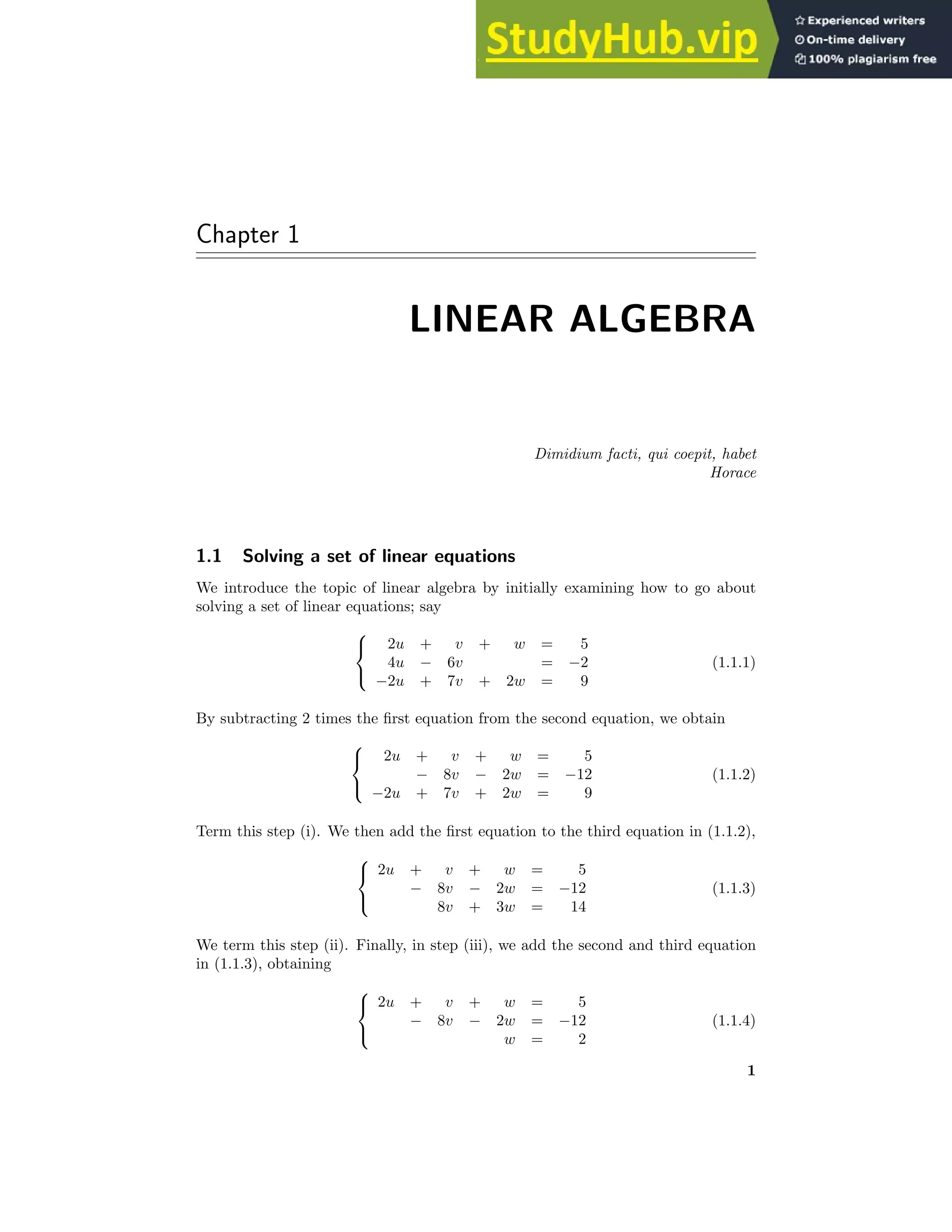
This procedure is known as Gaussian1
elimination, and from (1.1.4) we can easily
solve the equations via insertion, obtaining the solution (u, v, w) = (1, 1, 2). An
easy way to ensure that the found solution is correct is to simply insert (u, v, w)
in (1.1.1). However, we will normally prefer to work with matrices instead of the
above set of equations. The matrix approach offers many benefits, as well as opening
up a new way to view the equations, and we will here focus on matrices and the
geometries that can be associated with matrices.
1.2 Vectors and matrices
We proceed to write (1.1.1) on matrix form
2
4
−2
u +
1
−6
7
v +
1
0
2
w
| {z }
2
6
6
4
2 1 1
4 −6 0
−2 7 2
3
7
7
5
2
6
6
4
u
v
w
3
7
7
5
=
5
−2
9
(1.2.1)
Note that we can view the columns of the matrix as vectors in a three-dimensional
(real-valued) space, often written R3
. This is only to say that the elements of the
vectors can be viewed as the coordinates in a space, e.g., we view the third column
vector, say a3,
a3 =
1
0
2
(1.2.2)
as the vector starting at origin and ending at x = 1, y = 0 and z = 2. Using a
simplified geometric figure, we can depict the three column vectors as
✑
✑
✑
✑
✑
✑
✑
✑
✸
✲
✁
✁
✁
✁
✁
✁
✕ a2
a1
a3
where the vectors are seen as lying in a three-dimensional space. The solution
to the linear set of equations in (1.1.1) is thus the scalings (u, v, w) such that if we
1Johann Carl Friedrich Gauss (1777-1855) was born in Brunswick, the Duchy of Brunswick
(now Germany). In 1801, he received his doctorate in mathematics, proving the fundamental
theorem of algebra [7]. He made remarkable contributions to all fields of mathematics, and is
generally considered to be the greatest mathematician of all times.](https://image.slidesharecdn.com/anintroductiontolinearalgebra-230807170015-13d65227/75/An-Introduction-to-Linear-Algebra-pdf-5-2048.jpg)
![4 Linear Algebra Chapter 1
yielding (cf. 1.1.4))
2 1 1
0 −8 −2
0 0 1
u
v
w
=
5
−12
2
(1.2.9)
The resulting matrix, which we will term U, will be an upper-triangular matrix.
We denote the sought solution x =
u v w
T
, and note that we have by the
matrix multiplications rewritten
Ax = b ⇒ Ux = c, (1.2.10)
where U = (GFE) A and c = (GFE) b. As U is upper-triangular, the new matrix
equation is obviously trivial to solve via insertion.
We proceed by applying the inverses of the above elementary matrices (in reverse
order!), and note that
E−1
F−1
G−1
| {z }
L
GFEA
| {z }
U
= A. (1.2.11)
This is the so-called LU-decomposition, stating that
A square matrix that can be reduced to U (without row inter-
changes2
) can be written as A = LU.
As the inverse of an elementary matrix can be obtain by simply changing the sign
of the off-diagonal element3
,
E−1
=
1 0 0
−2 1 0
0 0 1
−1
=
1 0 0
2 1 0
0 0 1
(1.2.12)
we can immediately obtain the LU-decomposition after reducing A to U,
A = LU =
1 0 0
2 1 0
−1 −1 1
2 1 1
0 −8 −2
0 0 1
(1.2.13)
Note that L will be a lower-triangular matrix. Often, one divides out the diagonal
elements of U, the so-called pivots4
, denoting the diagonal matrix with the pivots
on the diagonal D, i.e.,
A = LU = LDŨ. (1.2.14)
2Note that in some cases, row exchanges are required to reduce A to U. In such case, A can
not be written as LU. See [1] for further details on row interchanges.
3Please note that this only holds for elementary matrices!
4We note that pivots are always nonzero.](https://image.slidesharecdn.com/anintroductiontolinearalgebra-230807170015-13d65227/75/An-Introduction-to-Linear-Algebra-pdf-7-2048.jpg)
![14 Linear Algebra Chapter 1
where the m × n matrix Q forms the orthonormal basis, and R is upper triangular
and invertible. This is the famous Q-R factorization. Note that A does not need
to be a square matrix to be written as in (1.4.20); however, if A is a square matrix,
then Q is a unitary matrix. In general:
If A ∈ Cm×n
, with m ≥ n, there is a matrix Q ∈ Cm×n
with
orthonormal columns and an upper triangular matrix R ∈ Cn×n
such that A = QR. If m = n, Q is unitary; if in addition A is
nonsingular, then R may be chosen so that all its diagonal entries
are positive. In this case, the factors Q and R are unique.
The Q-R factorization concludes our discussion on orthogonality, and we proceed
to dwell on the notion of determinants.
1.5 Determinants
As we have seen above, we often wish to know when a square matrix is invertible14
.
The simple answer is:
A matrix A is invertible, when the determinant of the matrix is
non-zero, i.e., det{A} 6= 0.
That is a good and short answer, but one that immediately raises another question.
What is then the determinant? This is less clear cut to answer, being somewhat
elusive. You might say that the determinant is a number that capture the soul of
a matrix, but for most this is a bit vague. Let us instead look at the definition of
the determinant; for a 2 by 2 matrix it is simple:
det
a11 a12
a21 a22
=
a11 a12
a21 a22
= a11a22 − a12a21 (1.5.1)
For a larger matrix, it is more of a mess. Then,
det A = ai1Ai1 + · · · + ainAin, (1.5.2)
where the cofactor Aij is
Aij = (−1)i+j
det Mij (1.5.3)
and the matrix Mij is formed by deleting row i and column j of A (see [1] for further
examples of the use of (1.5.2) and (1.5.3)). Often, one can use the properties of the
determinant to significantly simplify the calculations. The main properties are
(i) The determinant depends linearly on the first row.
a + a′
b + b′
c d
=
a b
c d
+
a′
b′
c d
(1.5.4)
14We note in passing that the inverse does not exist for non-square matrices; however, such
matrices might still have a left or a right inverse.](https://image.slidesharecdn.com/anintroductiontolinearalgebra-230807170015-13d65227/75/An-Introduction-to-Linear-Algebra-pdf-17-2048.jpg)
![Section 1.6. Eigendecomposition 15
(ii) The determinant change sign when two rows are exchanged.
a b
c d
= −
c d
a b
(1.5.5)
(iii) det I = 1.
Given these three basic properties, one can derive numerous determinant rules. We
will here only mention a few convenient rules, leaving the proofs to the interested
reader (see, e.g., [1,6]).
(iv) If two rows are equal, then det A = 0.
(v) If A has a zero row, then det A = 0.
(vi) Subtracting a multiple of one row from another leaves the det A unchanged.
(vii) If A is triangular, then det A is equal to the product of the main diagonal.
(viii) If A is singular, det A = 0.
(ix) det AB = (det A)(det B)
(x) det A = det AT
.
(xi) |cA| = cn
|A|, for c ∈ C.
(xii) det A−1
= (det A)
−1
.
(xiii) |I − AB| = |I − BA|.
where A, B ∈ Cn×n
. Noteworthy is that the determinant of a singular matrix is
zero. Thus, as long as the determinant of A is non-zero, the matrix A will be
non-singular and invertible. We will make immediate use of this fact.
1.6 Eigendecomposition
We now move to study eigenvalues and eigenvectors. Consider a square matrix A.
By definition, x is an eigenvector of A if it satisfies
Ax = λx. (1.6.1)
That is, if multiplied with A, it will only yield a scaled version of itself. Note that
(1.6.1) implies that
(A − λI) x = 0, (1.6.2)
requiring x to be in N(A−λI). We require that the eigenvector x must be non-zero,
and as a result, A − λI must be singular15
, i.e., the scaling λ is an eigenvalue of A
if and only if
det (A − λI) = 0. (1.6.3)
15Otherwise, the nullspace would not contain any vectors, leaving only x = 0 as a solution.](https://image.slidesharecdn.com/anintroductiontolinearalgebra-230807170015-13d65227/75/An-Introduction-to-Linear-Algebra-pdf-18-2048.jpg)
![Section 1.8. Total least squares 21
Comparing with (1.4.6), yields
A†
= Vӆ
UH
(1.7.10)
and the conclusion that the least squares solution can immediately be obtained
using the SVD. We also note that the singular values can be used to compute the
2-norm of a matrix,
kAk2 = σ1. (1.7.11)
As is clear from the above brief discussion, the SVD is a very powerful tool finding
use in numerous applications. We refer the interested reader to [3] and [4] for further
details on the theoretical and representational aspects of the SVD.
1.8 Total least squares
As an example of the use of the SVD, we will briefly touch on total least squares
(TLS). As mentioned in our earlier discussion on the least squares minimization, it
can be viewed as finding the vector x such that
min
x
kAx − bk2
2 (1.8.1)
Here, we are implicitly assuming that the errors are confined to the “observation”
vector b, such that
Ax = b + ∆b (1.8.2)
It is often relevant to also assume the existence of errors in the “data” matrix, i.e.,
(A + ∆A)x = (b + ∆b) (1.8.3)
Thus, we seek the vector x, such that (b + ∆b) ∈ R(A+∆A), which minimize the
norm of the perturbations. Geometrically, this can be viewed as finding the vector
x minimizing the (squared) total distance, as compared to finding the minimum
(squared) vertical distance; this is illustrated in the figure below for a line.
✲
✻
⋄
⋄
⋄
✲
✻
⋄
⋄
⋄
(a) LS: Minimize vertical (b) TLS: Minimize total
distance to line. distance to line.](https://image.slidesharecdn.com/anintroductiontolinearalgebra-230807170015-13d65227/75/An-Introduction-to-Linear-Algebra-pdf-24-2048.jpg)
![22 Linear Algebra Chapter 1
Let [A | B] denote the matrix obtained by concatenating the matrix A with the
matrix B, stacking the columns of B to the right of the columns of A. Note that,
0 =
A + ∆A | b + ∆b
x
−1
=
A | b
x
−1
+
∆A | ∆b
x
−1
(1.8.4)
and let
C =
A | b
D =
∆A | ∆b
(1.8.5)
Thus, in order for (1.8.4) to have a solution, the augmented vector [xT
, −1]T
must
lie in the nullspace of C + D, and in order for the solution to be non-trivial, the
perturbation D must be such that C + D is rank deficient19
. The TLS solution
finds the D with smallest norm that makes C + D rank deficient; put differently,
the TLS solution is the vector minimizing
min
∆A,∆b,x
k [∆A ∆b] k2
F such that (A + ∆A)x = b + ∆b (1.8.6)
where
kAk2
F = tr(AH
A) =
min (m,n)
X
k=1
σ2
k (1.8.7)
denotes the Frobenius norm, with σk being the kth singular value of A. Let C ∈
Cm×(n+1)
. Recalling (1.7.5), we write
C =
n+1
X
k=1
σkukvH
k (1.8.8)
The matrix of rank n closest to C can be shown to be the matrix formed using only
the n dominant singular values of C, i.e.,
C̃ =
n
X
k=1
σkukvH
k (1.8.9)
Thus, to ensure that C + D is rank deficient, we let
D = −σn+1un+1vH
n+1 (1.8.10)
19Recall that if C + D is full rank, the nullspace only contains the null vector.](https://image.slidesharecdn.com/anintroductiontolinearalgebra-230807170015-13d65227/75/An-Introduction-to-Linear-Algebra-pdf-25-2048.jpg)
![Section 1.8. Total least squares 23
For this choice of D, C + D does not contain the vector20
vn+1, and the solution
to (1.8.4) must thus be a multiple α of vn+1, i.e.,
x
−1
= αvn+1 (1.8.11)
yielding
xT LS = −
vn+1(1 : n)
vn+1(n + 1)
(1.8.12)
We note in passing that one can similarly write the solution to the TLS matrix
equation (A + ∆A)X = (B + ∆B), where B ∈ Cm×k
, as
XT LS = −V12V−1
22 (1.8.13)
if V−1
22 exists, where
V =
V11 V12
V21 V22
(1.8.14)
with V11 ∈ Cn×n
, V22 ∈ Ck×k
and V12, VT
21 ∈ Cn×k
. The TLS estimate yields a
strongly consistent estimate of the true solution when the errors in the concatenated
matrix [A b] are rowwise independently and identically distributed with zero mean
and equal variance. If, in addition, the errors are normally distributed, the TLS
solution has maximum likelihood properties. We refer the interested reader to [4]
and [5] for further details on theoretical and implementational aspects of the TLS.
20The vector vn+1 now lies in N (C + D).](https://image.slidesharecdn.com/anintroductiontolinearalgebra-230807170015-13d65227/75/An-Introduction-to-Linear-Algebra-pdf-26-2048.jpg)
![Appendix B
THE KARHUNEN-LOÈVE
TRANSFORM
E ne l’idolo suo si trasmutava
Dante
In this appendix, we will briefly describe the Karhunen-Loève transform (KLT).
Among all linear transforms, the KLT is the one which best approximates a stochas-
tic process in the least square sense. Furthermore, the coefficients of the KLT are
uncorrelated. These properties make the KLT very interesting for many signal pro-
cessing applications, such as coding and pattern recognition.
Let
xN = [x1, . . . , xN ]
T
(B.1.1)
be a zero-mean, stationary and ergodic random process with covariance matrix (see,
e.g., [8]).
Rxx = E{xN xH
N } (B.1.2)
where E{·} denotes the expectation operator. The eigenvalue problem
Rxxuj = λjuj, for j = 0, . . . , N − 1, (B.1.3)
yields the j:th eigenvalue, λj, as well as the j:th eigenvector, uj. Given that Rxx is
a covariance matrix1
, all eigenvalues will be real and non-negative (see also Section
1.6). Furthermore, N orthogonal eigenvectors can always be found, i.e.,
U = [u1, . . . , uN ] (B.1.4)
will be a unitary matrix. The KLT of xN is found as
α = UH
xN (B.1.5)
1A covariance matrix is always positive (semi) definite.
27](https://image.slidesharecdn.com/anintroductiontolinearalgebra-230807170015-13d65227/75/An-Introduction-to-Linear-Algebra-pdf-30-2048.jpg)
![28 The Karhunen-Loève transform Appendix B
where the KLT coefficients,
α = [α1, . . . , αN ]
T
, (B.1.6)
will be uncorrelated, i.e.,
E{αjαk} = λjδjk for j, k = 1, . . . , N. (B.1.7)
We note that this yields that
UH
RxxU = Λ ⇔ Rxx = UΛUH
(B.1.8)
where Λ = diag(λ1, . . . , λN ).](https://image.slidesharecdn.com/anintroductiontolinearalgebra-230807170015-13d65227/75/An-Introduction-to-Linear-Algebra-pdf-31-2048.jpg)
![BIBLIOGRAPHY
[1] G. Strang, Linear algebra and its applications, 3rd Ed. Thomson Learning, 1988.
[2] R. A. Horn and C. A. Johnson, Matrix Analysis. Cambridge, England: Cambridge
University Press, 1985.
[3] R. A. Horn and C. A. Johnson, Topics in Matrix Analysis. Cambridge, England:
Cambridge University Press, 1991.
[4] G. H. Golub and C. F. V. Loan, Matrix Computations (3rd edition). The John
Hopkins University Press, 1996.
[5] S. V. Huffel and J. Vandevalle, The Total Least Squares Problem: Computational
Aspects and Analysis. SIAM Publications, Philadelphia, 1991.
[6] P. Stoica and R. Moses, Introduction to Spectral Analysis. Upper Saddle River,
N.J.: Prentice Hall, 1997.
[7] J. C. F. Gauss, Demonstratio Nova Theorematis Omnem Functionem Alge-
braicam Rationalem Integram Unius Variabilis in Factores Reales Primi Vel Secundi
Gradus Resolve Posse. PhD thesis, University of Helmstedt, Germany, 1799.
[8] M. H. Hayes, Statistical Digital Signal Processing and Modeling. New York: John
Wiley and Sons, Inc., 1996.
30](https://image.slidesharecdn.com/anintroductiontolinearalgebra-230807170015-13d65227/75/An-Introduction-to-Linear-Algebra-pdf-33-2048.jpg)

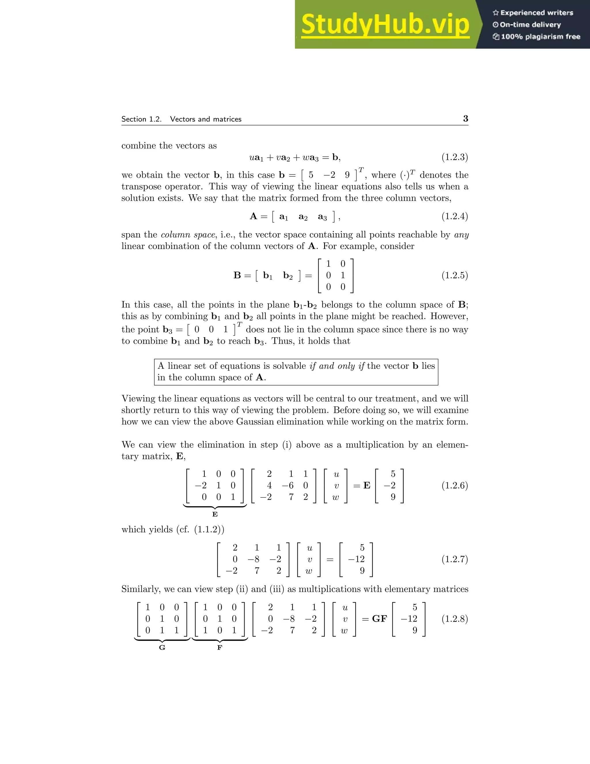
This document provides an introduction to linear algebra. It begins by demonstrating how to solve a system of linear equations using Gaussian elimination, and expresses this process using matrix multiplication and elementary matrices. It then introduces vectors and matrices, describing how a system of linear equations can be expressed as a matrix equation Ax=b. It explains that a solution exists if and only if the vector b lies in the column space of A. The document concludes by describing the LU decomposition, where a matrix A can be factored as A=LU, and how this decomposition can be used to efficiently solve systems of linear equations.