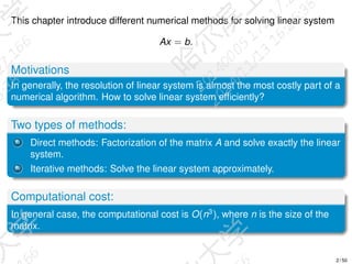
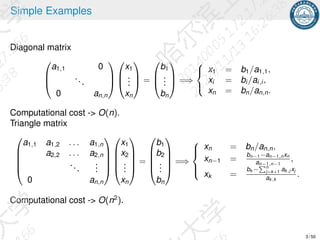
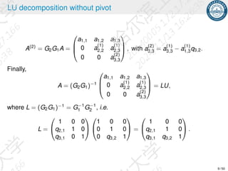
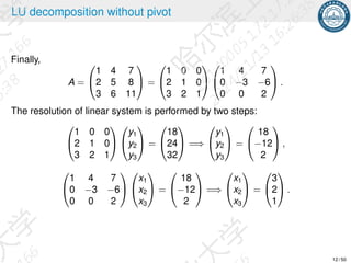
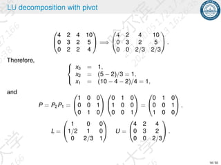
Resolution of Linear System
Chang YANG
School of Mathematics, Harbin Institute of Technology, Harbin, China
Autumn, Semester
1 / 50
This chapter introduce different numerical methods for solving linear system
Ax = b.
Motivations
In generally, the resolution of linear system is almost the most costly part of a
numerical algorithm. How to solve linear system efficiently?
Two types of methods:
(i)
Direct methods: Factorization of the matrix A and solve exactly the linear
system.
(ii)
Iterative methods: Solve the linear system approximately.
Computational cost:
In general case, the computational cost is O(n3
), where n is the size of the
matrix.
2 / 50
Simple Examples
Diagonal matrix



a1,1 0
...
0 an,n






x1
.
.
.
xn


 =



b1
.
.
.
bn


 =⇒



x1 = b1/a1,1,
xi = bi /ai,i ,
xn = bn/an,n.
Computational cost -> O(n).
Triangle matrix





a1,1 a1,2 . . . a1,n
a2,2 . . . a2,n
...
.
.
.
0 an,n










x1
x2
.
.
.
xn





=





b1
b2
.
.
.
bn





=⇒





xn = bn/an,n,
xn−1 =
bn−1−an−1,nxn
an−1,n−1
,
xk =
bk −
Pn
j=k+1 ak,j xj
ak,k
.
Computational cost -> O(n2
).
3 / 50
Outline
1 Direct Methods
2 Condition Number and Error for Resolution of Linear Systems
3 Classical Iterative Methods
4 / 50
Table of contents
1 Direct Methods
2 Condition Number and Error for Resolution of Linear Systems
3 Classical Iterative Methods
5 / 50
LU decomposition: General idea
The LU decomposition consists to factorize A as follows
PA = LU,
with
L =





1 0
l2,1 1
.
.
.
...
ln,1 . . . ln,n−1 1





and U =





u1,1 u1,2 . . . u1,n
u2,2 . . . u2,n
...
.
.
.
0 un,n





and P is a permutation matrix (P−1
= PT
).
Motivation: The resolution of linear system is made by two steps
LUx = Pb =⇒

Ly = Pb,
Ux = y.
6 / 50
LU decomposition without pivot
Hypothesis :
Assume all the principle matrices of A are invertible, i.e. det(Ak ) ̸= 0, with
Ak =



a1,1 . . . a1,k
.
.
.
.
.
.
ak,1 . . . ak,k


 , ∀k = 1, . . . , n.
Then there exists a decomposition LU with P = Id, i.e.
A = LU.
Example in dimension 3:
A =


a1,1 a1,2 a1,3
a2,1 a2,2 a2,3
a3,1 a3,2 a3,3

 , and

a1,1 = det(A1) ̸= 0,
a1,1a2,2 − a2,1a1,2 = det(A2) ̸= 0.
7 / 50
LU decomposition without pivot
With
G1 =


1 0 0
−q2,1 1 0
−q3,1 0 1

 , with
(
q2,1 =
a2,1
a1,1
,
q3,1 =
a3,1
a1,1
.
We have
A(1)
= G1A =



a1,1 a1,2 a1,3
0 a
(1)
2,2 a
(1)
2,3
0 a
(1)
3,2 a
(1)
3,3


 , with











a
(1)
2,2 = a2,2 − a1,2q2,1,
a
(1)
2,3 = a2,3 − a1,3q2,1,
a
(1)
3,2 = a3,2 − a1,2q3,1,
a
(1)
2,3 = a3,3 − a1,3q3,1.
We restart with A(1)
:
G2 =


1 0 0
0 1 0
0 −q3,2 1

 , with q3,2 =
a
(1)
3,2
a
(1)
2,2
.
8 / 50
LU decomposition without pivot
A(2)
= G2G1A =



a1,1 a1,2 a1,3
0 a
(1)
2,2 a
(1)
2,3
0 0 a
(2)
3,3


 , with a
(2)
3,3 = a
(1)
3,3 − a
(1)
1,3q3,2.
Finally,
A = (G2G1)−1



a1,1 a1,2 a1,3
0 a
(1)
2,2 a
(1)
2,3
0 0 a
(2)
3,3


 = LU,
where L = (G2G1)−1
= G−1
1 G−1
2 , i.e.
L =


1 0 0
q2,1 1 0
q3,1 0 1




1 0 0
0 1 0
0 q3,2 1

 =


1 0 0
q2,1 1 0
q3,1 q3,2 1

 .
9 / 50
LU decomposition without pivot
Algorithm: LU decomposition without pivot
for k = 1 : n − 1 do
for i = k + 1 : n do
qi,k = a
(k−1)
i,k /a
(k−1)
k,k
for j = k + 1 : n do
a
(k)
i,j = a
(k−1)
i,j − qi,k a
(k−1)
k,j
end for
end for
end for
Exercise
Compute the computational cost this algorithm.
10 / 50
LU decomposition without pivot
Example with
A =


1 4 7
2 5 8
3 6 11

 , and b =


18
24
32

 .
We compute q2,1 = a2,1/a1,1 = 2, q3,1 = a3,1/a1,1 = 3.


1 4 7 18
2 5 8 24
3 6 11 32

 =⇒


1 4 7 18
0 −3 −6 −12
0 −6 −10 −22

 .
Then we compute q3,2 = a
(1)
3,2/a
(1)
2,2 = 2.


1 4 7 18
0 −3 −6 −12
0 −6 −10 −22

 =⇒


1 4 7 18
0 −3 −6 −12
0 0 2 2

 .
11 / 50
LU decomposition without pivot
Finally,
A =


1 4 7
2 5 8
3 6 11

 =


1 0 0
2 1 0
3 2 1




1 4 7
0 −3 −6
0 0 2

 .
The resolution of linear system is performed by two steps:


1 0 0
2 1 0
3 2 1




y1
y2
y3

 =


18
24
32

 =⇒


y1
y2
y3

 =


18
−12
2

 ,


1 4 7
0 −3 −6
0 0 2




x1
x2
x3

 =


18
−12
2

 =⇒


x1
x2
x3

 =


3
2
1

 .
12 / 50
LU decomposition with pivot
Motivation
The LU decomposition is unstable when the coefficients a
(i)
i+1,i+1 is too small,
or the principle matrices are no longer invertible.
In practice, it is more efficient to use a LU decomposition with pivot.
Example with
A =


0 2 2
4 2 4
2 4 4

 , and b =


4
10
10

 .
We start by choosing the pivot, the largest element of the first column, then
we proceed the same LU algorithm without pivot.


0 2 2 4
4 2 4 10
2 4 4 10

 =⇒ P1 =


0 1 0
1 0 0
0 0 1

 =⇒


4 2 4 10
0 2 2 4
2 4 4 10

 ,


4 2 4 10
0 2 2 4
0 3 2 5

 =⇒ P2 =


1 0 0
0 0 1
0 1 0

 =⇒


4 2 4 10
0 3 2 5
0 2 2 4

 ,
13 / 50
LU decomposition with pivot


4 2 4 10
0 3 2 5
0 2 2 4

 =⇒


4 2 4 10
0 3 2 5
0 0 2/3 2/3

 .
Therefore, 


x3 = 1,
x2 = (5 − 2)/3 = 1,
x1 = (10 − 4 − 2)/4 = 1,
and
P = P2P1 =


1 0 0
0 0 1
0 1 0




0 1 0
1 0 0
0 0 1

 =


0 1 0
0 0 1
1 0 0

 ,
L =


1 0 0
1/2 1 0
0 2/3 1

 U =


4 2 4
0 3 2
0 0 2/3

 .
14 / 50
LU decomposition with pivot
The previous calculation yields
G2P2G1P1A = U.
By denoting M = G2P2G1P1, we have
MA = U,
MP−1
PA = U,
where P = P2P1. This implies
PA = (PM−1
)U.
Finally, L = PM−1
= P2P1P−1
1 G−1
1 P−1
2 G−1
2 = P2G−1
1 P−1
2 G−1
2 .
Exercise
Solve the linear system by using the LU decomposition with pivot
A =


3 1 6
2 1 3
1 1 1

 , and b =


2
4
7

 .
15 / 50
Cholesky Decomposition
The Cholesky decomposition consists to decompose the matrix A under the
form A = LLT
, where
L =





l1,1 0
l2,1 l2,2
.
.
.
...
ln,1 . . . ln,n−1 ln,n





Motivation
As the LU decomposition, the resolution of linear system Ax = b is performed
by two steps:
LLT
x = b =⇒

Ly = b,
LT
x = y.
The advantages with respect to the LU decomposition are
1 only have to store one matrix;
2 twice faster than the LU decomposition.
16 / 50
Cholesky Decomposition
Definition
A matrix A is positive definite if
 x, Ax ≥ 0 and  x, Ax = 0 =⇒ x = 0.
An example of such matrix are the diagonal strictly dominant matrices.
Theorem
If A is a symmetric positive definite matrix, then there are a unique inferior
triangular matrix L with positive diagonal coefficients such that
A = LLT
.
17 / 50
Cholesky Decomposition
Example in dimension 2
Let A =

a c
c b

be a positive definite matrix.
In particular, the hypothesis of positivity implies that

a = e1, Ae1   0,
ab − c2
= det(A)  0.
With
L =

l1,1 0
l2,1 l2,2

and LLT
=

l2
1,1 l1,1l2,1
l2,1l1,1 l2
2,1 + l2
2,2

.
We thus reduce that 




l1,1 =
√
a,
l2,1 = c
√
a
,
l2,2 =
q
b − c2
a .
18 / 50
Cholesky Decomposition
In general case,




l1,1 0
l2,1 l2,2
.
.
.
...
ln,1 . . . ln,n−1 ln,n









l1,1 l2,1 . . . ln,1
l2,2
.
.
.
... ln,n−1
0 ln,n





=





a1,1 a1,2 . . . a1,n
a1,2 a2,2
.
.
.
.
.
.
... an−1,n
a1,n . . . an−1,n an,n





.
The first row implies that a1,i = l1,1li,1 and



l1,1 =
√
a1,1,
li,1 =
a1,i
l1,1
, for i  1.
Thus, the first column is obtained.
The second row implies that a2,i = l2,1li,1 + l2,2li,2, for i ≥ 2 and



l2,2 =
q
a2,2 − l2
2,1,
li,2 =
a2,i −l2,1li,1
l2,2
, for i  2.
Thus, the second column is obtained.
19 / 50
Cholesky Decomposition




l1,1 0
l2,1 l2,2
.
.
.
...
ln,1 . . . ln,n−1 ln,n









l1,1 l2,1 . . . ln,1
l2,2
.
.
.
... ln,n−1
0 ln,n





=





a1,1 a1,2 . . . a1,n
a1,2 a2,2
.
.
.
.
.
.
... an−1,n
a1,n . . . an−1,n an,n





.
At the kth row, the k − 1 first columns of L are known, then
ak,i =
k
X
j=1
lk,j li,j , for i ≥ k
and 




lk,k =
q
ak,k −
Pk−1
j=1 l2
k,j ,
li,k =
ak,i −
Pk−1
j=1
lk,j li,j
lk,k
, for i  k.
Thus, the kth column of L is obtained.
20 / 50
Cholesky Decomposition
Algorithm: Cholesky Decomposition
for k = 1 : n − 1 do
lk,k =
q
ak,k −
Pk−1
j=1 l2
k,j
for i = k + 1 : n do
li,k =
ak,i −
Pk−1
j=1
lk,j li,j
lk,k
end for
end for
Exercise
Compute the computational cost this algorithm.
Exercise
Apply the algorithm of Cholesky to decompose the matrix
A =


4 2 1
2 4 2
1 2 4

 .
21 / 50
Table of contents
1 Direct Methods
2 Condition Number and Error for Resolution of Linear Systems
3 Classical Iterative Methods
22 / 50
The condition number of a matrix
Motivation
How an error δA of matrix A and an error δb of a vector b affect the solution x
of the linear system
Ax = b.
In particular, by denoting x + δx, the solution of linear system
(A + δA)(x + δx) = b + δb,
we expect to control the relative error
∥δx∥
∥x∥
.
23 / 50
Vectorial Norm
Definition
∥ · ∥ is a norm in Rn
verifying that if ∀(x, y) ∈ (Rn
)2
and α ∈ R, then
Positivity : ∥x∥  0 and ∥x∥ = 0 ⇐⇒ x = 0.
Linearity : ∥αx∥ = |α|∥x∥.
Triangular Inequality : ∥x + y∥ ≤ ∥x∥ + ∥y∥.
Example :
∥x∥2 =
qPn
i=1 x2
i .
∥x∥1 =
Pn
i=1 |xi |.
∥x∥∞ = maxi=1:n{|xi |}.
24 / 50
Matrix Norm
Definition
Let ∥ · ∥ be a norm in Rn
. We denote ||| · ||| an associated norm of matrix
space Rn×n
defined by
|||A||| = max
∥x∥≤1
||Ax|| = max
∥x∥
||Ax||
∥x∥
.
Exercise
Prove that ||| · ||| is a norm in matrix space Rn×n
.
Example :
|||A|||2 =
√
λmax, where λmax is the largest eigenvalue of the matrix AT
A.
|||A|||1 = maxj=1:n
Pn
i=1 |ai,j |.
|||A|||∞ = maxi=1:n
Pn
j=1 |ai,j |.
25 / 50
Condition Number
Definition
Let A ∈ Rn×n
be an invertible matrix. The condition number associated with a
given norm is defined by
cond(A) = |||A||| · |||A−1
|||.
Exercise
Compute condition number associated to the norm ∥ · ∥∞ of the matrix
A =

1.2969 0.8648
0.2161 0.1441

.
26 / 50
Condition Number
Theorem
Let x and x + δx be the solution of the linear systems
Ax = b,
A(x + δx) = b + δb.
Then
∥δx∥
∥x∥
≤ cond(A)
∥δb∥
∥b∥
.
Proof :
It is sufficient to remark that
Ax = b =⇒ ∥b∥ ≤ |||A||| · ∥x∥ =⇒ 1
∥x∥ ≤ |||A|||
∥b∥ .
Aδx = δb =⇒ ∥δx∥ ≤ |||A−1
||| · ∥δb∥.
27 / 50
Condition Number
Theorem
Let x and x + δx be the solution of the linear systems
Ax = b,
(A + δA)(x + δx) = b + δb.
Assume that |||A−1
||| · |||δA|||  1. Then
∥δx∥
∥x∥
≤
cond(A)
1 − |||A||| · |||δA|||

∥δb∥
∥b∥
+
|||δA|||
|||A|||

.
Proof :
By introducing δx = δxb + δxA, where
Aδxb = δb,
it yields that
Ax = b =⇒ ∥b∥ ≤ |||A||| · ∥x∥ =⇒
1
∥x∥
≤
|||A|||
∥b∥
,
Aδxb = δb =⇒ ∥δxb∥ ≤ |||A−1
||| · ∥δb∥,
28 / 50
Condition Number
and
(A + δA)(x + δxb + δxA) = b + δb =⇒ δxA = −A−1
δA(x + δx)
=⇒ ∥δxA∥ ≤ |||A−1
||| · |||δA|||(∥x∥ + ∥δx∥).
We thus reduce that
∥δx∥ ≤ ∥δxA∥ + ∥δxb∥ ≤ |||A−1
||| · ∥δb∥ + |||A−1
||| · |||δA|||(∥x∥ + ∥δx∥),
and
∥δx∥ ≤
1
1 − |||A−1||| · |||δA|||
|||A−1
||| · ∥δb∥ + |||A−1
||| · |||δA|||∥x∥

.
29 / 50
Table of contents
1 Direct Methods
2 Condition Number and Error for Resolution of Linear Systems
3 Classical Iterative Methods
30 / 50
Classical Iterative Methods
Motivations :
The computational cost of the direct method is O(N3
).
Usually, the matrix A is sparse (which means the majority coefficients
are zeros). While the LU decomposition losses this property. Thus we
have to face the problem of storage.
Example:
31 / 50
Fixed point method
The principle is to search the solution x∗
of linear system
Ax = b,
as a fixed point of an application ϕ : Rn
→ Rn
:
ϕ(x∗
) = x∗
.
The fixed point algorithm constructs a xk defined by

x0 ∈ Rn
,
xk+1 = ϕ(xk ).
If the application ϕ is well chosen, then we have
lim
k→∞
xk = x∗
.
32 / 50
Example of 1 dimension
With the function of the form ϕ(x) = ax + b.
a  1 a  1
A necessary and sufficient condition for xk → x∗
is
|a|  1.
33 / 50
Contraction and existence of fixed point
Definition
An application ϕ : Rn
→ Rn
is a contraction for the norm ∥ · ∥, if there exists
λ  1 such that
∥ϕ(x) − ϕ(y)∥ ≤ λ∥x − y∥.
Theorem
Let ϕ : Rn
→ Rn
be a contraction and x0 ∈ Rn
. Then the sequence xk defined
by 
x0 ∈ Rn
,
xk+1 = ϕ(xk ).
converges to the unique fixed point x∗
. Moreover,
(i)
Estimation a posteriori ∥x∗
− xk ∥ ≤ 1
1−λ ∥xk − xk+1∥;
(ii)
Estimation a priori ∥x∗
− xk ∥ ≤ λk
1−λ ∥x0 − x1∥.
34 / 50
Contraction and existence of fixed point
Proof :
1 It is sufficient to remark that
∥x∗
− xk ∥ ≤ ∥x∗
− xk+1 + xk+1 − xk ∥ ≤ ∥x∗
− xk+1∥ + ∥xk+1 − xk ∥
≤ ∥ϕ(x∗
) − ϕ(xk )∥ + ∥xk+1 − xk ∥
≤ λ∥x∗
− xk ∥ + ∥xk+1 − xk ∥.
2 With the inequality (1), we have
∥x∗
− xk ∥ ≤
1
1 − λ
∥xk+1 − xk ∥ ≤
1
1 − λ
∥ϕ(xk ) − ϕ(xk−1)∥
≤
λ
1 − λ
∥xk − xk−1∥ ≤
λk
1 − λ
∥x1 − x0∥.
35 / 50
Algorithm with a precision ε
Algorithm (Fixed point method)
Given : x0 ∈ Rn
, ε  0.
x1 = ϕ(x0), k = 1.
while ∥xk − xk−1∥  cε do
xk+1 = ϕ(xk )
k = k + 1
end while
Exercise
How to choose cε such that the algorithm stops with a precision of ε?
36 / 50
Application for the resolution of linear system
We are interested in the applications ϕ of the form
ϕ(x) = M−1
(Nx + b)
where A = M − N.
Exercise
Prove that if x∗
is a fixed point of ϕ, then
Ax∗
= b.
The application ϕ is a contraction if
|||M−1
N|||  1.
We remark that xk+1 = ϕ(xk ) is the solution of linear system
Mxk+1 = Nxk + b.
Idea : choose M close to A and easy to inverse.
37 / 50
Jacobi Method
The Jacobi method uses
M = D, N = −L − U.
Exercise
Prove
(xk+1)i =
1
aii

bi −
n
X
j=1,j̸=i
ai,j (xk )j

 .
Theorem
If A is diagonal strictly dominant, then the Jacobi method converges.
Theorem
If A is symmetric, ai,i  0, i = 1, . . . n, then the Jacobi method converges if
and only if A and 2D − A are positive definite.
38 / 50
Jacobi Method
Exercise
Find the convergent condition of the Jacobi method for the linear system
Ax = b.
A =


1 a a
a 1 a
a a 1


The principal minors of matrix A is ∆1 = 1, ∆2 = 1 − a2
,
∆3 = (1 − a)2
(1 + 2a). A is positive definite iff ∆2  0 and ∆3  0, which is
equivalent to −1
2  a  1.
2D − A =


1 −a −a
−a 1 −a
−a −a 1


The principal minors of matrix 2D − A is ∆1 = 1, ∆2 = 1 − a2
,
∆3 = (1 + a)2
(1 − 2a). 2D − A is positive definite iff ∆2  0 and ∆3  0,
which is equivalent to −1  a  1
2 .
Conclusion : the Jacobi method converges iff a ∈ (−1
2 , 1
2 ).
39 / 50
Gauss-Seidel Method
The Gauss-Seidel method uses
M = D + L, N = −U.
Exercise
Prove
(xk+1)i =
1
aii

bi −
i−1
X
j=1
ai,j (xk+1)j −
n
X
j=i+1
ai,j (xk )j

 .
Theorem
If A is symmetric positive definite, then the Gauss-Seidel method converges.
Exercise
Consider again the previous exercise, find the convergent condition of the
Gauss-Seidel method for the linear system Ax = b.
40 / 50
Gradient Method
Hypothesis : A is symmetric positive definite.
The principle is to search the solution x∗
of the linear system
Ax = b,
as the minimum of the energy
J(x) =
1
2
 Ax, x  −  b, x ,
where  Ax, x = xT
Ax,  b, x = xT
b.
We construct then a sequence {xk }, which minimizes J as follows

x0 ∈ Rn
,
xk+1 = xk + αk rk , ∀k ≥ 1,
where rk is the descent direction and αk is the descent step.
41 / 50
Gradient Method
The choice of rk :
The direction rk is the opposite of the gradient of J, i.e.
rk = −∇J(xk ) = −(Axk − b) = b − Axk .
The choice of αk :
We choose αk as the step who minimizes J in the direction rk
J̃(α) = J(xk + αrk ).
With
J̃′
(α) = ∇J(xk + αrk ), rk 
= A(xk + αrk ) − b, rk 
= α  Ark , rk  −  rk , rk ,
we deduce that
J̃′
(α) = 0 ⇐⇒ αk =
 rk , rk 
 Ark , rk 
.
42 / 50
Gradient Method
Algorithm (Gradient method)
1: Given : x0 ∈ Rn
, ε  0.
2: while ∥Axk − b∥  ε|||A−1
||| do
3: rk = b − Axk
4: αk = rk , rk  /  Ark , rk 
5: xk+1 = xk + αk rk
6: end while
Example avec A = (1, 0; 0, 5), b = (0, 0)T
and x0 = (1, 0.2)T
.
43 / 50
Gradient Method
The drawback of the Gradient method:
Theorem
Assume the spectral of A is λ1 ≥ λ2 ≥ · · · ≥ λn  0, then we have
∥xk − x∗
∥A ≤

λ1 − λn
λ1 + λn
k
∥x0 − x∗
∥A
where ∥u∥A =
p
(Au, u).
When λ1 ≫ λn, the convergent rate of the gradient method is very slow.
44 / 50
Conjugate Gradient Method
Definition
Assume A positive definite, if {p0, p1, . . . , pn−1} is Rn
, satisfying
 Api , pj = 0, i ̸= j, then {p0, p1, . . . , pn−1} are A-conjugate.
Different from the gradient method, now we search the A-conjugate descent
directions.
Assume that the direction p0, p1, . . . , pk−1 are given and A-conjugate, we
search pk such that {p0, p1, . . . , pk } are A-conjugate. We decompose
x = y + αpk , where y ∈ span{p0, p1, . . . , pk−1}, α ∈ R.
J(x) = J(y + αpk )
= J(y) +
α2
2
 Apk , pk  −α  b, pk , (since  Ay, pk = 0)
min
x∈span{p0,p1,...,pk }
J(x) = min
y,α
J(y + αpk )
= min
y
J(y) + min
α
[
α2
2
 Apk , pk  −α  b, pk ].
45 / 50
Conjugate Gradient Method
The solution of min
y
J(y) is y = xk .
The solution of min
α
[
α2
2
 Apk , pk  −α  b, pk ] is
αk =
 b, pk 
 Apk , pk 
=
 b − Axk , pk 
 Apk , pk 
=
 rk , pk 
 Apk , pk 
.
Moreover, we assume that pk = rk + βk−1pk−1.
By using the fact  pk , Apk−1 = 0, we obtain
βk−1 = −
 rk , Apk−1 
 pk−1, Apk−1 
.
46 / 50
Conjugate Gradient Method
Algorithm (Conjugate Gradient method)
1: Given : x0 ∈ Rn
, ε  0, r0 = b − Ax0, p0 = r0.
2: while ∥Axk − b∥  ε|||A−1
||| do
3: αk = rk , pk  /  Apk , pk 
4: xk+1 = xk + αk pk
5: βk = −  rk+1, Apk  /  pk , Apk 
6: pk+1 = rk+1 + βk pk
7: end while
Example avec A = (1, 0; 0, 5), b = (0, 0)T
and x0 = (1, 0.2)T
.
47 / 50
Conjugate Gradient Method
Theorem
Assume the spectral of A is λ1 ≥ λ2 ≥ · · · ≥ λn  0, then we have
∥xk − x∗
∥A ≤ 2
√
λ1 −
√
λn
√
λ1 +
√
λn
k
∥x0 − x∗
∥A
where ∥u∥A =
√
 Au, u .
Compare to the gradient method, the conjugate gradient method is much
better.
However, when λ1 ≫ λn, the convergent rate of the conjugate gradient
method is still very slow.
48 / 50
Complementary Exercises
Exercise
Compute the LU decomposition of matrix A:
A =


6 4 2
3 −2 −1
3 4 1


Exercise
Compute the LU decomposition of matrix A:
A =


1 2 3
4 5 6
7 8 10


49 / 50
Complementary Exercises
Exercise
Compute the Cholesky decomposition of matrix A:
A =


4 2 1
2 3 1
1 1 4


Exercise
Solve the following linear system by the Jacobi method and the Gauss-Seidel
method 

10 −1 −2
−1 10 −2
−1 −1 5




x1
x2
x3

 =


72
83
42


50 / 50

Linear_system, Linear_system, Linear_system.pdf

  • 1.
    Resolution of LinearSystem Chang YANG School of Mathematics, Harbin Institute of Technology, Harbin, China Autumn, Semester 1 / 50
  • 2.
    This chapter introducedifferent numerical methods for solving linear system Ax = b. Motivations In generally, the resolution of linear system is almost the most costly part of a numerical algorithm. How to solve linear system efficiently? Two types of methods: (i) Direct methods: Factorization of the matrix A and solve exactly the linear system. (ii) Iterative methods: Solve the linear system approximately. Computational cost: In general case, the computational cost is O(n3 ), where n is the size of the matrix. 2 / 50
  • 3.
    Simple Examples Diagonal matrix    a1,10 ... 0 an,n       x1 . . . xn    =    b1 . . . bn    =⇒    x1 = b1/a1,1, xi = bi /ai,i , xn = bn/an,n. Computational cost -> O(n). Triangle matrix      a1,1 a1,2 . . . a1,n a2,2 . . . a2,n ... . . . 0 an,n           x1 x2 . . . xn      =      b1 b2 . . . bn      =⇒      xn = bn/an,n, xn−1 = bn−1−an−1,nxn an−1,n−1 , xk = bk − Pn j=k+1 ak,j xj ak,k . Computational cost -> O(n2 ). 3 / 50
  • 4.
    Outline 1 Direct Methods 2Condition Number and Error for Resolution of Linear Systems 3 Classical Iterative Methods 4 / 50
  • 5.
    Table of contents 1Direct Methods 2 Condition Number and Error for Resolution of Linear Systems 3 Classical Iterative Methods 5 / 50
  • 6.
    LU decomposition: Generalidea The LU decomposition consists to factorize A as follows PA = LU, with L =      1 0 l2,1 1 . . . ... ln,1 . . . ln,n−1 1      and U =      u1,1 u1,2 . . . u1,n u2,2 . . . u2,n ... . . . 0 un,n      and P is a permutation matrix (P−1 = PT ). Motivation: The resolution of linear system is made by two steps LUx = Pb =⇒ Ly = Pb, Ux = y. 6 / 50
  • 7.
    LU decomposition withoutpivot Hypothesis : Assume all the principle matrices of A are invertible, i.e. det(Ak ) ̸= 0, with Ak =    a1,1 . . . a1,k . . . . . . ak,1 . . . ak,k    , ∀k = 1, . . . , n. Then there exists a decomposition LU with P = Id, i.e. A = LU. Example in dimension 3: A =   a1,1 a1,2 a1,3 a2,1 a2,2 a2,3 a3,1 a3,2 a3,3   , and a1,1 = det(A1) ̸= 0, a1,1a2,2 − a2,1a1,2 = det(A2) ̸= 0. 7 / 50
  • 8.
    LU decomposition withoutpivot With G1 =   1 0 0 −q2,1 1 0 −q3,1 0 1   , with ( q2,1 = a2,1 a1,1 , q3,1 = a3,1 a1,1 . We have A(1) = G1A =    a1,1 a1,2 a1,3 0 a (1) 2,2 a (1) 2,3 0 a (1) 3,2 a (1) 3,3    , with            a (1) 2,2 = a2,2 − a1,2q2,1, a (1) 2,3 = a2,3 − a1,3q2,1, a (1) 3,2 = a3,2 − a1,2q3,1, a (1) 2,3 = a3,3 − a1,3q3,1. We restart with A(1) : G2 =   1 0 0 0 1 0 0 −q3,2 1   , with q3,2 = a (1) 3,2 a (1) 2,2 . 8 / 50
  • 9.
    LU decomposition withoutpivot A(2) = G2G1A =    a1,1 a1,2 a1,3 0 a (1) 2,2 a (1) 2,3 0 0 a (2) 3,3    , with a (2) 3,3 = a (1) 3,3 − a (1) 1,3q3,2. Finally, A = (G2G1)−1    a1,1 a1,2 a1,3 0 a (1) 2,2 a (1) 2,3 0 0 a (2) 3,3    = LU, where L = (G2G1)−1 = G−1 1 G−1 2 , i.e. L =   1 0 0 q2,1 1 0 q3,1 0 1     1 0 0 0 1 0 0 q3,2 1   =   1 0 0 q2,1 1 0 q3,1 q3,2 1   . 9 / 50
  • 10.
    LU decomposition withoutpivot Algorithm: LU decomposition without pivot for k = 1 : n − 1 do for i = k + 1 : n do qi,k = a (k−1) i,k /a (k−1) k,k for j = k + 1 : n do a (k) i,j = a (k−1) i,j − qi,k a (k−1) k,j end for end for end for Exercise Compute the computational cost this algorithm. 10 / 50
  • 11.
    LU decomposition withoutpivot Example with A =   1 4 7 2 5 8 3 6 11   , and b =   18 24 32   . We compute q2,1 = a2,1/a1,1 = 2, q3,1 = a3,1/a1,1 = 3.   1 4 7 18 2 5 8 24 3 6 11 32   =⇒   1 4 7 18 0 −3 −6 −12 0 −6 −10 −22   . Then we compute q3,2 = a (1) 3,2/a (1) 2,2 = 2.   1 4 7 18 0 −3 −6 −12 0 −6 −10 −22   =⇒   1 4 7 18 0 −3 −6 −12 0 0 2 2   . 11 / 50
  • 12.
    LU decomposition withoutpivot Finally, A =   1 4 7 2 5 8 3 6 11   =   1 0 0 2 1 0 3 2 1     1 4 7 0 −3 −6 0 0 2   . The resolution of linear system is performed by two steps:   1 0 0 2 1 0 3 2 1     y1 y2 y3   =   18 24 32   =⇒   y1 y2 y3   =   18 −12 2   ,   1 4 7 0 −3 −6 0 0 2     x1 x2 x3   =   18 −12 2   =⇒   x1 x2 x3   =   3 2 1   . 12 / 50
  • 13.
    LU decomposition withpivot Motivation The LU decomposition is unstable when the coefficients a (i) i+1,i+1 is too small, or the principle matrices are no longer invertible. In practice, it is more efficient to use a LU decomposition with pivot. Example with A =   0 2 2 4 2 4 2 4 4   , and b =   4 10 10   . We start by choosing the pivot, the largest element of the first column, then we proceed the same LU algorithm without pivot.   0 2 2 4 4 2 4 10 2 4 4 10   =⇒ P1 =   0 1 0 1 0 0 0 0 1   =⇒   4 2 4 10 0 2 2 4 2 4 4 10   ,   4 2 4 10 0 2 2 4 0 3 2 5   =⇒ P2 =   1 0 0 0 0 1 0 1 0   =⇒   4 2 4 10 0 3 2 5 0 2 2 4   , 13 / 50
  • 14.
    LU decomposition withpivot   4 2 4 10 0 3 2 5 0 2 2 4   =⇒   4 2 4 10 0 3 2 5 0 0 2/3 2/3   . Therefore,    x3 = 1, x2 = (5 − 2)/3 = 1, x1 = (10 − 4 − 2)/4 = 1, and P = P2P1 =   1 0 0 0 0 1 0 1 0     0 1 0 1 0 0 0 0 1   =   0 1 0 0 0 1 1 0 0   , L =   1 0 0 1/2 1 0 0 2/3 1   U =   4 2 4 0 3 2 0 0 2/3   . 14 / 50
  • 15.
    LU decomposition withpivot The previous calculation yields G2P2G1P1A = U. By denoting M = G2P2G1P1, we have MA = U, MP−1 PA = U, where P = P2P1. This implies PA = (PM−1 )U. Finally, L = PM−1 = P2P1P−1 1 G−1 1 P−1 2 G−1 2 = P2G−1 1 P−1 2 G−1 2 . Exercise Solve the linear system by using the LU decomposition with pivot A =   3 1 6 2 1 3 1 1 1   , and b =   2 4 7   . 15 / 50
  • 16.
    Cholesky Decomposition The Choleskydecomposition consists to decompose the matrix A under the form A = LLT , where L =      l1,1 0 l2,1 l2,2 . . . ... ln,1 . . . ln,n−1 ln,n      Motivation As the LU decomposition, the resolution of linear system Ax = b is performed by two steps: LLT x = b =⇒ Ly = b, LT x = y. The advantages with respect to the LU decomposition are 1 only have to store one matrix; 2 twice faster than the LU decomposition. 16 / 50
  • 17.
    Cholesky Decomposition Definition A matrixA is positive definite if x, Ax ≥ 0 and x, Ax = 0 =⇒ x = 0. An example of such matrix are the diagonal strictly dominant matrices. Theorem If A is a symmetric positive definite matrix, then there are a unique inferior triangular matrix L with positive diagonal coefficients such that A = LLT . 17 / 50
  • 18.
    Cholesky Decomposition Example indimension 2 Let A = a c c b be a positive definite matrix. In particular, the hypothesis of positivity implies that a = e1, Ae1 0, ab − c2 = det(A) 0. With L = l1,1 0 l2,1 l2,2 and LLT = l2 1,1 l1,1l2,1 l2,1l1,1 l2 2,1 + l2 2,2 . We thus reduce that      l1,1 = √ a, l2,1 = c √ a , l2,2 = q b − c2 a . 18 / 50
  • 19.
    Cholesky Decomposition In generalcase,     l1,1 0 l2,1 l2,2 . . . ... ln,1 . . . ln,n−1 ln,n          l1,1 l2,1 . . . ln,1 l2,2 . . . ... ln,n−1 0 ln,n      =      a1,1 a1,2 . . . a1,n a1,2 a2,2 . . . . . . ... an−1,n a1,n . . . an−1,n an,n      . The first row implies that a1,i = l1,1li,1 and    l1,1 = √ a1,1, li,1 = a1,i l1,1 , for i 1. Thus, the first column is obtained. The second row implies that a2,i = l2,1li,1 + l2,2li,2, for i ≥ 2 and    l2,2 = q a2,2 − l2 2,1, li,2 = a2,i −l2,1li,1 l2,2 , for i 2. Thus, the second column is obtained. 19 / 50
  • 20.
    Cholesky Decomposition     l1,1 0 l2,1l2,2 . . . ... ln,1 . . . ln,n−1 ln,n          l1,1 l2,1 . . . ln,1 l2,2 . . . ... ln,n−1 0 ln,n      =      a1,1 a1,2 . . . a1,n a1,2 a2,2 . . . . . . ... an−1,n a1,n . . . an−1,n an,n      . At the kth row, the k − 1 first columns of L are known, then ak,i = k X j=1 lk,j li,j , for i ≥ k and      lk,k = q ak,k − Pk−1 j=1 l2 k,j , li,k = ak,i − Pk−1 j=1 lk,j li,j lk,k , for i k. Thus, the kth column of L is obtained. 20 / 50
  • 21.
    Cholesky Decomposition Algorithm: CholeskyDecomposition for k = 1 : n − 1 do lk,k = q ak,k − Pk−1 j=1 l2 k,j for i = k + 1 : n do li,k = ak,i − Pk−1 j=1 lk,j li,j lk,k end for end for Exercise Compute the computational cost this algorithm. Exercise Apply the algorithm of Cholesky to decompose the matrix A =   4 2 1 2 4 2 1 2 4   . 21 / 50
  • 22.
    Table of contents 1Direct Methods 2 Condition Number and Error for Resolution of Linear Systems 3 Classical Iterative Methods 22 / 50
  • 23.
    The condition numberof a matrix Motivation How an error δA of matrix A and an error δb of a vector b affect the solution x of the linear system Ax = b. In particular, by denoting x + δx, the solution of linear system (A + δA)(x + δx) = b + δb, we expect to control the relative error ∥δx∥ ∥x∥ . 23 / 50
  • 24.
    Vectorial Norm Definition ∥ ·∥ is a norm in Rn verifying that if ∀(x, y) ∈ (Rn )2 and α ∈ R, then Positivity : ∥x∥ 0 and ∥x∥ = 0 ⇐⇒ x = 0. Linearity : ∥αx∥ = |α|∥x∥. Triangular Inequality : ∥x + y∥ ≤ ∥x∥ + ∥y∥. Example : ∥x∥2 = qPn i=1 x2 i . ∥x∥1 = Pn i=1 |xi |. ∥x∥∞ = maxi=1:n{|xi |}. 24 / 50
  • 25.
    Matrix Norm Definition Let ∥· ∥ be a norm in Rn . We denote ||| · ||| an associated norm of matrix space Rn×n defined by |||A||| = max ∥x∥≤1 ||Ax|| = max ∥x∥ ||Ax|| ∥x∥ . Exercise Prove that ||| · ||| is a norm in matrix space Rn×n . Example : |||A|||2 = √ λmax, where λmax is the largest eigenvalue of the matrix AT A. |||A|||1 = maxj=1:n Pn i=1 |ai,j |. |||A|||∞ = maxi=1:n Pn j=1 |ai,j |. 25 / 50
  • 26.
    Condition Number Definition Let A∈ Rn×n be an invertible matrix. The condition number associated with a given norm is defined by cond(A) = |||A||| · |||A−1 |||. Exercise Compute condition number associated to the norm ∥ · ∥∞ of the matrix A = 1.2969 0.8648 0.2161 0.1441 . 26 / 50
  • 27.
    Condition Number Theorem Let xand x + δx be the solution of the linear systems Ax = b, A(x + δx) = b + δb. Then ∥δx∥ ∥x∥ ≤ cond(A) ∥δb∥ ∥b∥ . Proof : It is sufficient to remark that Ax = b =⇒ ∥b∥ ≤ |||A||| · ∥x∥ =⇒ 1 ∥x∥ ≤ |||A||| ∥b∥ . Aδx = δb =⇒ ∥δx∥ ≤ |||A−1 ||| · ∥δb∥. 27 / 50
  • 28.
    Condition Number Theorem Let xand x + δx be the solution of the linear systems Ax = b, (A + δA)(x + δx) = b + δb. Assume that |||A−1 ||| · |||δA||| 1. Then ∥δx∥ ∥x∥ ≤ cond(A) 1 − |||A||| · |||δA||| ∥δb∥ ∥b∥ + |||δA||| |||A||| . Proof : By introducing δx = δxb + δxA, where Aδxb = δb, it yields that Ax = b =⇒ ∥b∥ ≤ |||A||| · ∥x∥ =⇒ 1 ∥x∥ ≤ |||A||| ∥b∥ , Aδxb = δb =⇒ ∥δxb∥ ≤ |||A−1 ||| · ∥δb∥, 28 / 50
  • 29.
    Condition Number and (A +δA)(x + δxb + δxA) = b + δb =⇒ δxA = −A−1 δA(x + δx) =⇒ ∥δxA∥ ≤ |||A−1 ||| · |||δA|||(∥x∥ + ∥δx∥). We thus reduce that ∥δx∥ ≤ ∥δxA∥ + ∥δxb∥ ≤ |||A−1 ||| · ∥δb∥ + |||A−1 ||| · |||δA|||(∥x∥ + ∥δx∥), and ∥δx∥ ≤ 1 1 − |||A−1||| · |||δA||| |||A−1 ||| · ∥δb∥ + |||A−1 ||| · |||δA|||∥x∥ . 29 / 50
  • 30.
    Table of contents 1Direct Methods 2 Condition Number and Error for Resolution of Linear Systems 3 Classical Iterative Methods 30 / 50
  • 31.
    Classical Iterative Methods Motivations: The computational cost of the direct method is O(N3 ). Usually, the matrix A is sparse (which means the majority coefficients are zeros). While the LU decomposition losses this property. Thus we have to face the problem of storage. Example: 31 / 50
  • 32.
    Fixed point method Theprinciple is to search the solution x∗ of linear system Ax = b, as a fixed point of an application ϕ : Rn → Rn : ϕ(x∗ ) = x∗ . The fixed point algorithm constructs a xk defined by x0 ∈ Rn , xk+1 = ϕ(xk ). If the application ϕ is well chosen, then we have lim k→∞ xk = x∗ . 32 / 50
  • 33.
    Example of 1dimension With the function of the form ϕ(x) = ax + b. a 1 a 1 A necessary and sufficient condition for xk → x∗ is |a| 1. 33 / 50
  • 34.
    Contraction and existenceof fixed point Definition An application ϕ : Rn → Rn is a contraction for the norm ∥ · ∥, if there exists λ 1 such that ∥ϕ(x) − ϕ(y)∥ ≤ λ∥x − y∥. Theorem Let ϕ : Rn → Rn be a contraction and x0 ∈ Rn . Then the sequence xk defined by x0 ∈ Rn , xk+1 = ϕ(xk ). converges to the unique fixed point x∗ . Moreover, (i) Estimation a posteriori ∥x∗ − xk ∥ ≤ 1 1−λ ∥xk − xk+1∥; (ii) Estimation a priori ∥x∗ − xk ∥ ≤ λk 1−λ ∥x0 − x1∥. 34 / 50
  • 35.
    Contraction and existenceof fixed point Proof : 1 It is sufficient to remark that ∥x∗ − xk ∥ ≤ ∥x∗ − xk+1 + xk+1 − xk ∥ ≤ ∥x∗ − xk+1∥ + ∥xk+1 − xk ∥ ≤ ∥ϕ(x∗ ) − ϕ(xk )∥ + ∥xk+1 − xk ∥ ≤ λ∥x∗ − xk ∥ + ∥xk+1 − xk ∥. 2 With the inequality (1), we have ∥x∗ − xk ∥ ≤ 1 1 − λ ∥xk+1 − xk ∥ ≤ 1 1 − λ ∥ϕ(xk ) − ϕ(xk−1)∥ ≤ λ 1 − λ ∥xk − xk−1∥ ≤ λk 1 − λ ∥x1 − x0∥. 35 / 50
  • 36.
    Algorithm with aprecision ε Algorithm (Fixed point method) Given : x0 ∈ Rn , ε 0. x1 = ϕ(x0), k = 1. while ∥xk − xk−1∥ cε do xk+1 = ϕ(xk ) k = k + 1 end while Exercise How to choose cε such that the algorithm stops with a precision of ε? 36 / 50
  • 37.
    Application for theresolution of linear system We are interested in the applications ϕ of the form ϕ(x) = M−1 (Nx + b) where A = M − N. Exercise Prove that if x∗ is a fixed point of ϕ, then Ax∗ = b. The application ϕ is a contraction if |||M−1 N||| 1. We remark that xk+1 = ϕ(xk ) is the solution of linear system Mxk+1 = Nxk + b. Idea : choose M close to A and easy to inverse. 37 / 50
  • 38.
    Jacobi Method The Jacobimethod uses M = D, N = −L − U. Exercise Prove (xk+1)i = 1 aii  bi − n X j=1,j̸=i ai,j (xk )j   . Theorem If A is diagonal strictly dominant, then the Jacobi method converges. Theorem If A is symmetric, ai,i 0, i = 1, . . . n, then the Jacobi method converges if and only if A and 2D − A are positive definite. 38 / 50
  • 39.
    Jacobi Method Exercise Find theconvergent condition of the Jacobi method for the linear system Ax = b. A =   1 a a a 1 a a a 1   The principal minors of matrix A is ∆1 = 1, ∆2 = 1 − a2 , ∆3 = (1 − a)2 (1 + 2a). A is positive definite iff ∆2 0 and ∆3 0, which is equivalent to −1 2 a 1. 2D − A =   1 −a −a −a 1 −a −a −a 1   The principal minors of matrix 2D − A is ∆1 = 1, ∆2 = 1 − a2 , ∆3 = (1 + a)2 (1 − 2a). 2D − A is positive definite iff ∆2 0 and ∆3 0, which is equivalent to −1 a 1 2 . Conclusion : the Jacobi method converges iff a ∈ (−1 2 , 1 2 ). 39 / 50
  • 40.
    Gauss-Seidel Method The Gauss-Seidelmethod uses M = D + L, N = −U. Exercise Prove (xk+1)i = 1 aii  bi − i−1 X j=1 ai,j (xk+1)j − n X j=i+1 ai,j (xk )j   . Theorem If A is symmetric positive definite, then the Gauss-Seidel method converges. Exercise Consider again the previous exercise, find the convergent condition of the Gauss-Seidel method for the linear system Ax = b. 40 / 50
  • 41.
    Gradient Method Hypothesis :A is symmetric positive definite. The principle is to search the solution x∗ of the linear system Ax = b, as the minimum of the energy J(x) = 1 2 Ax, x − b, x , where Ax, x = xT Ax, b, x = xT b. We construct then a sequence {xk }, which minimizes J as follows x0 ∈ Rn , xk+1 = xk + αk rk , ∀k ≥ 1, where rk is the descent direction and αk is the descent step. 41 / 50
  • 42.
    Gradient Method The choiceof rk : The direction rk is the opposite of the gradient of J, i.e. rk = −∇J(xk ) = −(Axk − b) = b − Axk . The choice of αk : We choose αk as the step who minimizes J in the direction rk J̃(α) = J(xk + αrk ). With J̃′ (α) = ∇J(xk + αrk ), rk = A(xk + αrk ) − b, rk = α Ark , rk − rk , rk , we deduce that J̃′ (α) = 0 ⇐⇒ αk = rk , rk Ark , rk . 42 / 50
  • 43.
    Gradient Method Algorithm (Gradientmethod) 1: Given : x0 ∈ Rn , ε 0. 2: while ∥Axk − b∥ ε|||A−1 ||| do 3: rk = b − Axk 4: αk = rk , rk / Ark , rk 5: xk+1 = xk + αk rk 6: end while Example avec A = (1, 0; 0, 5), b = (0, 0)T and x0 = (1, 0.2)T . 43 / 50
  • 44.
    Gradient Method The drawbackof the Gradient method: Theorem Assume the spectral of A is λ1 ≥ λ2 ≥ · · · ≥ λn 0, then we have ∥xk − x∗ ∥A ≤ λ1 − λn λ1 + λn k ∥x0 − x∗ ∥A where ∥u∥A = p (Au, u). When λ1 ≫ λn, the convergent rate of the gradient method is very slow. 44 / 50
  • 45.
    Conjugate Gradient Method Definition AssumeA positive definite, if {p0, p1, . . . , pn−1} is Rn , satisfying Api , pj = 0, i ̸= j, then {p0, p1, . . . , pn−1} are A-conjugate. Different from the gradient method, now we search the A-conjugate descent directions. Assume that the direction p0, p1, . . . , pk−1 are given and A-conjugate, we search pk such that {p0, p1, . . . , pk } are A-conjugate. We decompose x = y + αpk , where y ∈ span{p0, p1, . . . , pk−1}, α ∈ R. J(x) = J(y + αpk ) = J(y) + α2 2 Apk , pk −α b, pk , (since Ay, pk = 0) min x∈span{p0,p1,...,pk } J(x) = min y,α J(y + αpk ) = min y J(y) + min α [ α2 2 Apk , pk −α b, pk ]. 45 / 50
  • 46.
    Conjugate Gradient Method Thesolution of min y J(y) is y = xk . The solution of min α [ α2 2 Apk , pk −α b, pk ] is αk = b, pk Apk , pk = b − Axk , pk Apk , pk = rk , pk Apk , pk . Moreover, we assume that pk = rk + βk−1pk−1. By using the fact pk , Apk−1 = 0, we obtain βk−1 = − rk , Apk−1 pk−1, Apk−1 . 46 / 50
  • 47.
    Conjugate Gradient Method Algorithm(Conjugate Gradient method) 1: Given : x0 ∈ Rn , ε 0, r0 = b − Ax0, p0 = r0. 2: while ∥Axk − b∥ ε|||A−1 ||| do 3: αk = rk , pk / Apk , pk 4: xk+1 = xk + αk pk 5: βk = − rk+1, Apk / pk , Apk 6: pk+1 = rk+1 + βk pk 7: end while Example avec A = (1, 0; 0, 5), b = (0, 0)T and x0 = (1, 0.2)T . 47 / 50
  • 48.
    Conjugate Gradient Method Theorem Assumethe spectral of A is λ1 ≥ λ2 ≥ · · · ≥ λn 0, then we have ∥xk − x∗ ∥A ≤ 2 √ λ1 − √ λn √ λ1 + √ λn k ∥x0 − x∗ ∥A where ∥u∥A = √ Au, u . Compare to the gradient method, the conjugate gradient method is much better. However, when λ1 ≫ λn, the convergent rate of the conjugate gradient method is still very slow. 48 / 50
  • 49.
    Complementary Exercises Exercise Compute theLU decomposition of matrix A: A =   6 4 2 3 −2 −1 3 4 1   Exercise Compute the LU decomposition of matrix A: A =   1 2 3 4 5 6 7 8 10   49 / 50
  • 50.
    Complementary Exercises Exercise Compute theCholesky decomposition of matrix A: A =   4 2 1 2 3 1 1 1 4   Exercise Solve the following linear system by the Jacobi method and the Gauss-Seidel method   10 −1 −2 −1 10 −2 −1 −1 5     x1 x2 x3   =   72 83 42   50 / 50