Preface
Here are my online notes for my Linear Algebra course that I teach here at Lamar University.
Despite the fact that these are my “class notes”, they should be accessible to anyone wanting to
learn Linear Algebra or needing a refresher.
These notes do assume that the reader has a good working knowledge of basic Algebra. This set
of notes is fairly self contained but there is enough Algebra type problems (arithmetic and
occasionally solving equations) that can show up that not having a good background in Algebra
can cause the occasional problem.
Here are a couple of warnings to my students who may be here to get a copy of what happened on
a day that you missed.
1. Because I wanted to make this a fairly complete set of notes for anyone wanting to learn
Linear Algebra I have included some material that I do not usually have time to cover in
class and because this changes from semester to semester it is not noted here. You will
need to find one of your fellow class mates to see if there is something in these notes that
wasn’t covered in class.
2. In general I try to work problems in class that are different from my notes. However,
with a Linear Algebra course while I can make up the problems off the top of my head
there is no guarantee that they will work out nicely or the way I want them to. So,
because of that my class work will tend to follow these notes fairly close as far as worked
problems go. With that being said I will, on occasion, work problems off the top of my
head when I can to provide more examples than just those in my notes. Also, I often
don’t have time in class to work all of the problems in the notes and so you will find that
some sections contain problems that weren’t worked in class due to time restrictions.
3. Sometimes questions in class will lead down paths that are not covered here. I try to
anticipate as many of the questions as possible in writing these notes up, but the reality is
that I can’t anticipate all the questions. Sometimes a very good question gets asked in
class that leads to insights that I’ve not included here. You should always talk to
someone who was in class on the day you missed and compare these notes to their notes
and see what the differences are.
4. This is somewhat related to the previous three items, but is important enough to merit its
own item. THESE NOTES ARE NOT A SUBSTITUTE FOR ATTENDING CLASS!!
Using these notes as a substitute for class is liable to get you in trouble. As already noted
not everything in these notes is covered in class and often material or insights not in these
notes is covered in class.
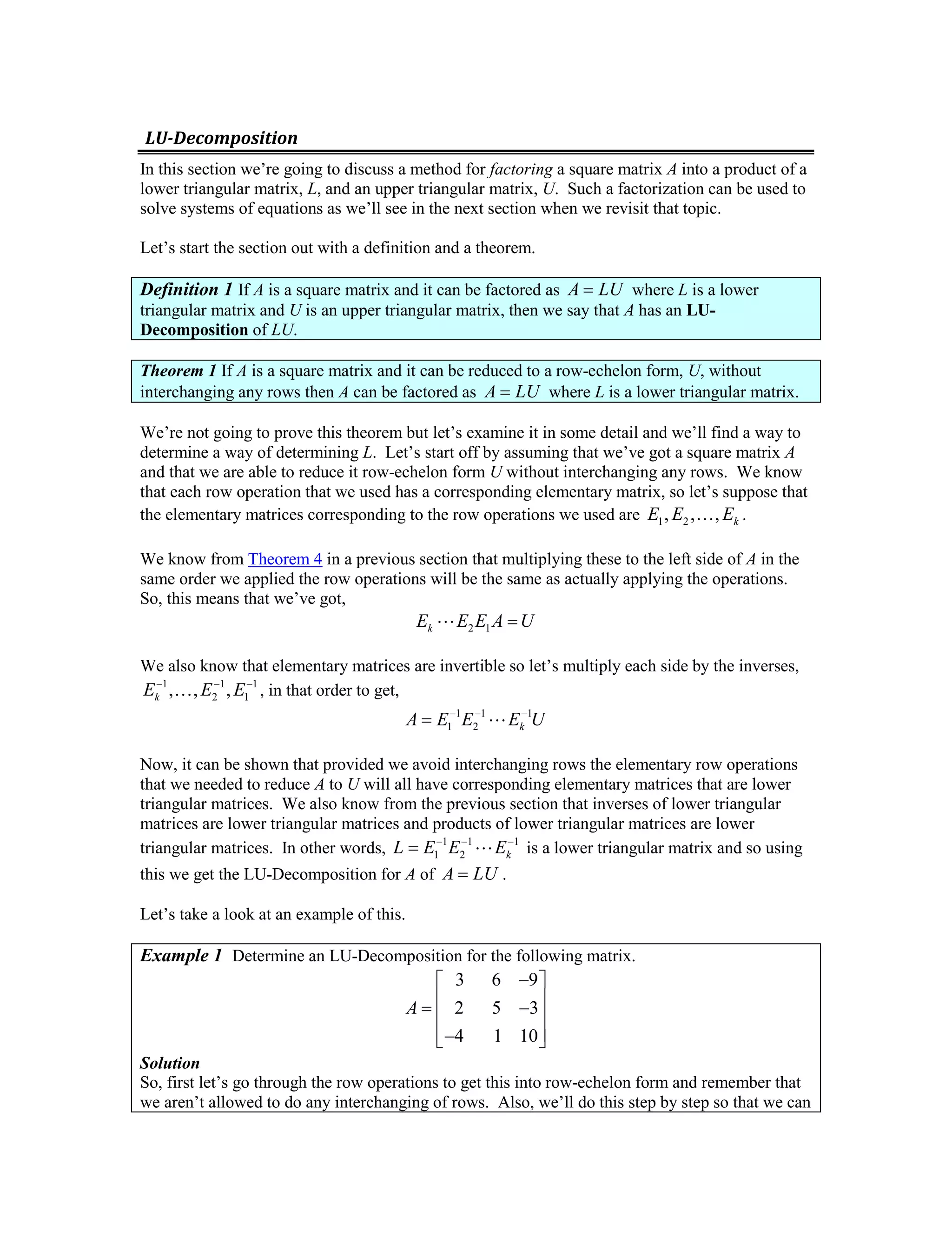
LU-Decomposition
In this section we’re going to discuss a method for factoring a square matrix A into a product of a
lower triangular matrix, L, and an upper triangular matrix, U. Such a factorization can be used to
solve systems of equations as we’ll see in the next section when we revisit that topic.
Let’s start the section out with a definition and a theorem.
Definition 1 If A is a square matrix and it can be factored as A LU= where L is a lower
triangular matrix and U is an upper triangular matrix, then we say that A has an LU-
Decomposition of LU.
Theorem 1 If A is a square matrix and it can be reduced to a row-echelon form, U, without
interchanging any rows then A can be factored as A LU= where L is a lower triangular matrix.
We’re not going to prove this theorem but let’s examine it in some detail and we’ll find a way to
determine a way of determining L. Let’s start off by assuming that we’ve got a square matrix A
and that we are able to reduce it row-echelon form U without interchanging any rows. We know
that each row operation that we used has a corresponding elementary matrix, so let’s suppose that
the elementary matrices corresponding to the row operations we used are 1 2, , , kE E EK .
We know from Theorem 4 in a previous section that multiplying these to the left side of A in the
same order we applied the row operations will be the same as actually applying the operations.
So, this means that we’ve got,
2 1kE E E A U=L
We also know that elementary matrices are invertible so let’s multiply each side by the inverses,
1 1 1
2 1, , ,kE E E- - -
K , in that order to get,
1 1 1
1 2 kA E E E U- - -
= L
Now, it can be shown that provided we avoid interchanging rows the elementary row operations
that we needed to reduce A to U will all have corresponding elementary matrices that are lower
triangular matrices. We also know from the previous section that inverses of lower triangular
matrices are lower triangular matrices and products of lower triangular matrices are lower
triangular matrices. In other words, 1 1 1
1 2 kL E E E- - -
= L is a lower triangular matrix and so using
this we get the LU-Decomposition for A of A LU= .
Let’s take a look at an example of this.
Example 1 Determine an LU-Decomposition for the following matrix.
3 6 9
2 5 3
4 1 10
A
-é ù
ê ú= -ê ú
ê ú-ë û
Solution
So, first let’s go through the row operations to get this into row-echelon form and remember that
we aren’t allowed to do any interchanging of rows. Also, we’ll do this step by step so that we can
keep track of the row operations that we used since we’re going to need to write down the
elementary matrices that are associated with them eventually.
1
13
3 6 9 1 2 3
2 5 3 2 5 3
4 1 10 4 1 10
R
- -é ù é ù
ê ú ê ú- -ê ú ê ú®
ê ú ê ú- -ë û ë û
2 1
1 2 3 1 2 3
2
2 5 3 0 1 3
4 1 10 4 1 10
R R
- -é ù é ù
-ê ú ê ú-ê ú ê ú®
ê ú ê ú- -ë û ë û
3 1
1 2 3 1 2 3
4
0 1 3 0 1 3
4 1 10 0 9 2
R R
- -é ù é ù
+ê ú ê ú
ê ú ê ú®
ê ú ê ú- -ë û ë û
3 2
1 2 3 1 2 3
9
0 1 3 0 1 3
0 9 2 0 0 29
R R
- -é ù é ù
-ê ú ê ú
ê ú ê ú®
ê ú ê ú- -ë û ë û
1
329
1 2 3 1 2 3
0 1 3 0 1 3
0 0 29 0 0 1
R
- -é ù é ù
-ê ú ê ú
ê ú ê ú®
ê ú ê ú-ë û ë û
Okay so, we’ve got our hands on U.
1 2 3
0 1 3
0 0 1
U
-é ù
ê ú= ê ú
ê úë û
Now we need to get L. This is going to take a little more work. We’ll need the elementary
matrices for each of these, or more precisely their inverses. Recall that we can get the elementary
matrix for a particular row operation by applying that operation to the appropriately sized identity
matrix (3 3´ in this case). Also recall that the inverse matrix can be found by applying the
inverse operation to the identity matrix.
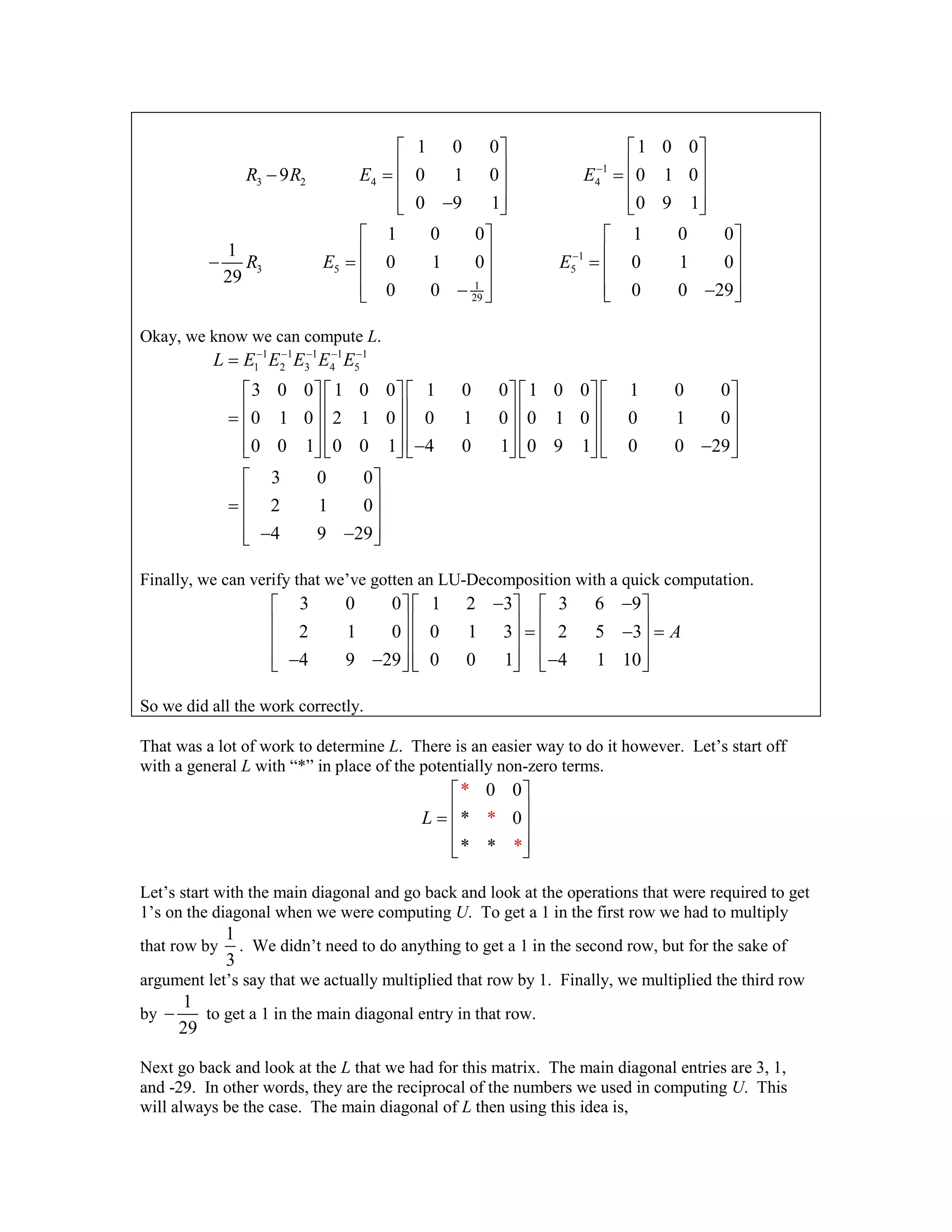
Here are the elementary matrices and their inverses for each of the operations above.
1
3
1
1 1 1
0 0 3 0 0
1
0 1 0 0 1 0
3
0 0 1 0 0 1
R E E-
é ù é ù
ê ú ê ú= =ê ú ê ú
ê ú ê úë ûë û
1
2 1 2 2
1 0 0 1 0 0
2 2 1 0 2 1 0
0 0 1 0 0 1
R R E E-
é ù é ù
ê ú ê ú- = - =ê ú ê ú
ê ú ê úë û ë û
1
3 1 3 3
1 0 0 1 0 0
4 0 1 0 0 1 0
4 0 1 4 0 1
R R E E-
é ù é ù
ê ú ê ú+ = =ê ú ê ú
ê ú ê ú-ë û ë û
1
3 2 4 4
1 0 0 1 0 0
9 0 1 0 0 1 0
0 9 1 0 9 1
R R E E-
é ù é ù
ê ú ê ú- = =ê ú ê ú
ê ú ê ú-ë û ë û
1
3 5 5
1
29
1 0 0 1 0 0
1
0 1 0 0 1 0
29
0 0 0 0 29
R E E-
é ù é ù
ê ú ê ú- = =ê ú ê ú
ê ú ê ú- -ë ûë û
Okay, we know we can compute L.
1 1 1 1 1
1 2 3 4 5
3 0 0 1 0 0 1 0 0 1 0 0 1 0 0
0 1 0 2 1 0 0 1 0 0 1 0 0 1 0
0 0 1 0 0 1 4 0 1 0 9 1 0 0 29
3 0 0
2 1 0
4 9 29
L E E E E E- - - - -
=
é ù é ù é ù é ù é ù
ê ú ê ú ê ú ê ú ê ú= ê ú ê ú ê ú ê ú ê ú
ê ú ê ú ê ú ê ú ê ú- -ë û ë û ë û ë û ë û
é ù
ê ú= ê ú
ê ú- -ë û
Finally, we can verify that we’ve gotten an LU-Decomposition with a quick computation.
3 0 0 1 2 3 3 6 9
2 1 0 0 1 3 2 5 3
4 9 29 0 0 1 4 1 10
A
- -é ù é ù é ù
ê ú ê ú ê ú= - =ê ú ê ú ê ú
ê ú ê ú ê ú- - -ë û ë û ë û
So we did all the work correctly.
That was a lot of work to determine L. There is an easier way to do it however. Let’s start off
with a general L with “*” in place of the potentially non-zero terms.
*
*
*
0 0
* 0
* *
L
é ù
ê ú= ê ú
ê úë û
Let’s start with the main diagonal and go back and look at the operations that were required to get
1’s on the diagonal when we were computing U. To get a 1 in the first row we had to multiply
that row by
1
3
. We didn’t need to do anything to get a 1 in the second row, but for the sake of
argument let’s say that we actually multiplied that row by 1. Finally, we multiplied the third row
by
1
29
- to get a 1 in the main diagonal entry in that row.
Next go back and look at the L that we had for this matrix. The main diagonal entries are 3, 1,
and -29. In other words, they are the reciprocal of the numbers we used in computing U. This
will always be the case. The main diagonal of L then using this idea is,
3 0 0
1 0
* 2
*
* 9
L
é ù
ê ú= ê ú
ê ú-ë û
Now, let’s take a look at the two entries under the 3 in the first column. Again go back to the
operations used to find U and take a look at the operations we used to get zeroes in these two
spots. To get a zero in the second row we added 12R- onto 2R and to get a zero in the third row
we added 14R onto 3R .
Again, go back to the L we found and notice that these two entries are 2 and -4. Or, they are the
negative of the multiple of the first row that we added onto that particular row to get that entry to
be zero. Filling these in we now arrive at,
3 0 0
2 1 0
4 29*
L
é ù
ê ú= ê ú
ê ú- -ë û
Finally, in determining U we aded 29R- onto 3R to get the entry in the third row and second
column to be zero and in the L we found this entry is 9. Again, it’s the negative of the multiple of
the second row we used to make this entry zero. This gives us the final entry in L.
3 0 0
2 1 0
4 9 29
L
é ù
ê ú= ê ú
ê ú- -ë û
This process we just went through will always work in determining L for our LU-Decomposition
provided we follow the process above to find U. In fact that is the one drawback to this process.
We need to find U using exactly the same steps we used in this example. In other words,
multiply/divide the first row by an appropriate scalar to get a 1 in the first column then zero out
the entries below that one. Next, multiply/divide the second row by an appropriate scalar to get a
1 in the main diagonal entry of the second row and then zero out all the entries below this.
Continue in this fashion until you’ve dealt with all the columns. This will sometimes lead to
some messy fractions.
Let’s take a look at another example and this time we’ll use the procedure outlined above to find
L instead of dealing with all the elementary matrices.
Example 2 Determine an LU-Decomposition for the following matrix.
2 3 4
5 4 4
1 7 0
B
-é ù
ê ú= ê ú
ê ú-ë û
Solution
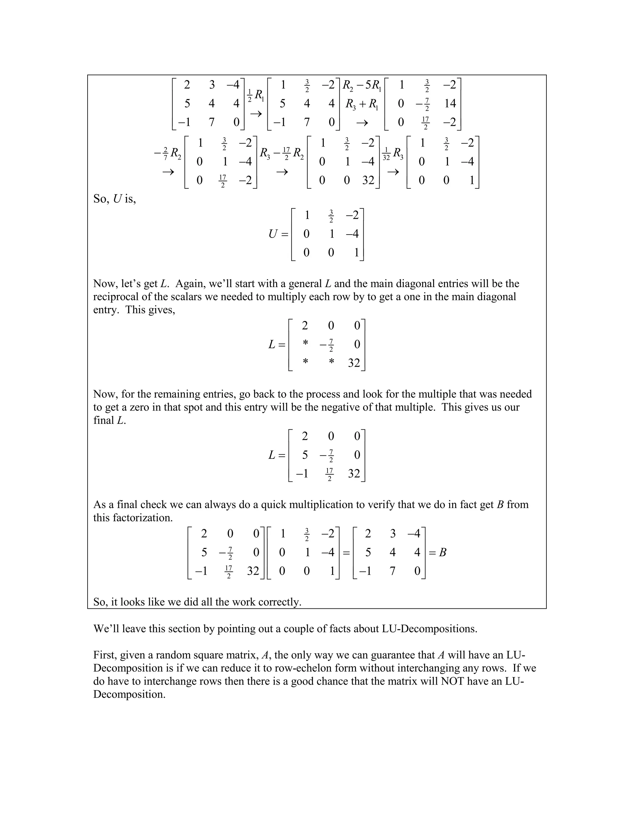
So, we first need to reduce B to row-echelon form without using row interchanges. Also, if we’re
going to use the process outlined above to find L we’ll need to do the reduction in the same
manner as the first example. Here is that work.
3 3
2 12 21
12 7
3 1 2
17
2
2 3 4 1 2 5 1 2
5 4 4 5 4 4 0 14
1 7 0 1 7 0 0 2
R R
R
R R
- - - -é ù é ùé ù
ê ú ê úê ú + -ê ú ê úê ú ®
ê ú ê úê ú- - ® -ë û ë û ë û
3 3 3
2 2 2172 1
2 33 27 322
17
2
1 2 1 2 1 2
0 1 4 0 1 4 0 1 4
0 2 0 0 32 0 0 1
R RR R
- - -é ù é ù é ù
- -ê ú ê ú ê ú- - -ê ú ê ú ê ú® ®®
ê ú ê ú ê ú-ë û ë û ë û
So, U is,
3
21 2
0 1 4
0 0 1
U
-é ù
ê ú= -ê ú
ê úë û
Now, let’s get L. Again, we’ll start with a general L and the main diagonal entries will be the
reciprocal of the scalars we needed to multiply each row by to get a one in the main diagonal
entry. This gives,
7
2
2 0 0
* 0
* * 32
L
é ù
ê ú= -ê ú
ê úë û
Now, for the remaining entries, go back to the process and look for the multiple that was needed
to get a zero in that spot and this entry will be the negative of that multiple. This gives us our
final L.
7
2
17
2
2 0 0
5 0
1 32
L
é ù
ê ú= -ê ú
ê ú-ë û
As a final check we can always do a quick multiplication to verify that we do in fact get B from
this factorization.
3
2
7
2
17
2
2 0 0 1 2 2 3 4
5 0 0 1 4 5 4 4
1 32 0 0 1 1 7 0
B
- -é ùé ù é ù
ê úê ú ê ú- - = =ê úê ú ê ú
ê úê ú ê ú- -ë ûë û ë û
So, it looks like we did all the work correctly.
We’ll leave this section by pointing out a couple of facts about LU-Decompositions.
First, given a random square matrix, A, the only way we can guarantee that A will have an LU-
Decomposition is if we can reduce it to row-echelon form without interchanging any rows. If we
do have to interchange rows then there is a good chance that the matrix will NOT have an LU-
Decomposition.
Second, notice that every time we’ve talked about an LU-Decomposition of a matrix we’ve used
the word “an” and not “the” LU-Decomposition. This choice of words is intentional. As the
choice suggests there is no single unique LU-Decomposition for A.
To see that LU-Decompositions are not unique go back to the first example. In that example we
computed the following LU-Decomposition.
3 6 9 3 0 0 1 2 3
2 5 3 2 1 0 0 1 3
4 1 10 4 9 29 0 0 1
- -é ù é ù é ù
ê ú ê ú ê ú- =ê ú ê ú ê ú
ê ú ê ú ê ú- - -ë û ë û ë û
However, we’ve also got the following LU-Decomposition.
2
3
4
3
3 6 9 1 0 0 3 6 9
2 5 3 1 0 0 1 3
4 1 10 9 1 0 0 29
- -é ùé ù é ù
ê úê ú ê ú- = ê úê ú ê ú
ê úê ú ê ú- - -ë û ë ûë û
This is clearly an LU-Decomposition since the first matrix is lower triangular and the second is
upper triangular and you should verify that upon multiplying they do in fact give the shown
matrix.
If you would like to see a further example of an LU-Decomposition worked out there is an
example in the next section.

Lu decomposition

  • 1.
    Preface Here are myonline notes for my Linear Algebra course that I teach here at Lamar University. Despite the fact that these are my “class notes”, they should be accessible to anyone wanting to learn Linear Algebra or needing a refresher. These notes do assume that the reader has a good working knowledge of basic Algebra. This set of notes is fairly self contained but there is enough Algebra type problems (arithmetic and occasionally solving equations) that can show up that not having a good background in Algebra can cause the occasional problem. Here are a couple of warnings to my students who may be here to get a copy of what happened on a day that you missed. 1. Because I wanted to make this a fairly complete set of notes for anyone wanting to learn Linear Algebra I have included some material that I do not usually have time to cover in class and because this changes from semester to semester it is not noted here. You will need to find one of your fellow class mates to see if there is something in these notes that wasn’t covered in class. 2. In general I try to work problems in class that are different from my notes. However, with a Linear Algebra course while I can make up the problems off the top of my head there is no guarantee that they will work out nicely or the way I want them to. So, because of that my class work will tend to follow these notes fairly close as far as worked problems go. With that being said I will, on occasion, work problems off the top of my head when I can to provide more examples than just those in my notes. Also, I often don’t have time in class to work all of the problems in the notes and so you will find that some sections contain problems that weren’t worked in class due to time restrictions. 3. Sometimes questions in class will lead down paths that are not covered here. I try to anticipate as many of the questions as possible in writing these notes up, but the reality is that I can’t anticipate all the questions. Sometimes a very good question gets asked in class that leads to insights that I’ve not included here. You should always talk to someone who was in class on the day you missed and compare these notes to their notes and see what the differences are. 4. This is somewhat related to the previous three items, but is important enough to merit its own item. THESE NOTES ARE NOT A SUBSTITUTE FOR ATTENDING CLASS!! Using these notes as a substitute for class is liable to get you in trouble. As already noted not everything in these notes is covered in class and often material or insights not in these notes is covered in class.
  • 2.
    LU-Decomposition In this sectionwe’re going to discuss a method for factoring a square matrix A into a product of a lower triangular matrix, L, and an upper triangular matrix, U. Such a factorization can be used to solve systems of equations as we’ll see in the next section when we revisit that topic. Let’s start the section out with a definition and a theorem. Definition 1 If A is a square matrix and it can be factored as A LU= where L is a lower triangular matrix and U is an upper triangular matrix, then we say that A has an LU- Decomposition of LU. Theorem 1 If A is a square matrix and it can be reduced to a row-echelon form, U, without interchanging any rows then A can be factored as A LU= where L is a lower triangular matrix. We’re not going to prove this theorem but let’s examine it in some detail and we’ll find a way to determine a way of determining L. Let’s start off by assuming that we’ve got a square matrix A and that we are able to reduce it row-echelon form U without interchanging any rows. We know that each row operation that we used has a corresponding elementary matrix, so let’s suppose that the elementary matrices corresponding to the row operations we used are 1 2, , , kE E EK . We know from Theorem 4 in a previous section that multiplying these to the left side of A in the same order we applied the row operations will be the same as actually applying the operations. So, this means that we’ve got, 2 1kE E E A U=L We also know that elementary matrices are invertible so let’s multiply each side by the inverses, 1 1 1 2 1, , ,kE E E- - - K , in that order to get, 1 1 1 1 2 kA E E E U- - - = L Now, it can be shown that provided we avoid interchanging rows the elementary row operations that we needed to reduce A to U will all have corresponding elementary matrices that are lower triangular matrices. We also know from the previous section that inverses of lower triangular matrices are lower triangular matrices and products of lower triangular matrices are lower triangular matrices. In other words, 1 1 1 1 2 kL E E E- - - = L is a lower triangular matrix and so using this we get the LU-Decomposition for A of A LU= . Let’s take a look at an example of this. Example 1 Determine an LU-Decomposition for the following matrix. 3 6 9 2 5 3 4 1 10 A -é ù ê ú= -ê ú ê ú-ë û Solution So, first let’s go through the row operations to get this into row-echelon form and remember that we aren’t allowed to do any interchanging of rows. Also, we’ll do this step by step so that we can
  • 3.
    keep track ofthe row operations that we used since we’re going to need to write down the elementary matrices that are associated with them eventually. 1 13 3 6 9 1 2 3 2 5 3 2 5 3 4 1 10 4 1 10 R - -é ù é ù ê ú ê ú- -ê ú ê ú® ê ú ê ú- -ë û ë û 2 1 1 2 3 1 2 3 2 2 5 3 0 1 3 4 1 10 4 1 10 R R - -é ù é ù -ê ú ê ú-ê ú ê ú® ê ú ê ú- -ë û ë û 3 1 1 2 3 1 2 3 4 0 1 3 0 1 3 4 1 10 0 9 2 R R - -é ù é ù +ê ú ê ú ê ú ê ú® ê ú ê ú- -ë û ë û 3 2 1 2 3 1 2 3 9 0 1 3 0 1 3 0 9 2 0 0 29 R R - -é ù é ù -ê ú ê ú ê ú ê ú® ê ú ê ú- -ë û ë û 1 329 1 2 3 1 2 3 0 1 3 0 1 3 0 0 29 0 0 1 R - -é ù é ù -ê ú ê ú ê ú ê ú® ê ú ê ú-ë û ë û Okay so, we’ve got our hands on U. 1 2 3 0 1 3 0 0 1 U -é ù ê ú= ê ú ê úë û Now we need to get L. This is going to take a little more work. We’ll need the elementary matrices for each of these, or more precisely their inverses. Recall that we can get the elementary matrix for a particular row operation by applying that operation to the appropriately sized identity matrix (3 3´ in this case). Also recall that the inverse matrix can be found by applying the inverse operation to the identity matrix. Here are the elementary matrices and their inverses for each of the operations above. 1 3 1 1 1 1 0 0 3 0 0 1 0 1 0 0 1 0 3 0 0 1 0 0 1 R E E- é ù é ù ê ú ê ú= =ê ú ê ú ê ú ê úë ûë û 1 2 1 2 2 1 0 0 1 0 0 2 2 1 0 2 1 0 0 0 1 0 0 1 R R E E- é ù é ù ê ú ê ú- = - =ê ú ê ú ê ú ê úë û ë û 1 3 1 3 3 1 0 0 1 0 0 4 0 1 0 0 1 0 4 0 1 4 0 1 R R E E- é ù é ù ê ú ê ú+ = =ê ú ê ú ê ú ê ú-ë û ë û
  • 4.
    1 3 2 44 1 0 0 1 0 0 9 0 1 0 0 1 0 0 9 1 0 9 1 R R E E- é ù é ù ê ú ê ú- = =ê ú ê ú ê ú ê ú-ë û ë û 1 3 5 5 1 29 1 0 0 1 0 0 1 0 1 0 0 1 0 29 0 0 0 0 29 R E E- é ù é ù ê ú ê ú- = =ê ú ê ú ê ú ê ú- -ë ûë û Okay, we know we can compute L. 1 1 1 1 1 1 2 3 4 5 3 0 0 1 0 0 1 0 0 1 0 0 1 0 0 0 1 0 2 1 0 0 1 0 0 1 0 0 1 0 0 0 1 0 0 1 4 0 1 0 9 1 0 0 29 3 0 0 2 1 0 4 9 29 L E E E E E- - - - - = é ù é ù é ù é ù é ù ê ú ê ú ê ú ê ú ê ú= ê ú ê ú ê ú ê ú ê ú ê ú ê ú ê ú ê ú ê ú- -ë û ë û ë û ë û ë û é ù ê ú= ê ú ê ú- -ë û Finally, we can verify that we’ve gotten an LU-Decomposition with a quick computation. 3 0 0 1 2 3 3 6 9 2 1 0 0 1 3 2 5 3 4 9 29 0 0 1 4 1 10 A - -é ù é ù é ù ê ú ê ú ê ú= - =ê ú ê ú ê ú ê ú ê ú ê ú- - -ë û ë û ë û So we did all the work correctly. That was a lot of work to determine L. There is an easier way to do it however. Let’s start off with a general L with “*” in place of the potentially non-zero terms. * * * 0 0 * 0 * * L é ù ê ú= ê ú ê úë û Let’s start with the main diagonal and go back and look at the operations that were required to get 1’s on the diagonal when we were computing U. To get a 1 in the first row we had to multiply that row by 1 3 . We didn’t need to do anything to get a 1 in the second row, but for the sake of argument let’s say that we actually multiplied that row by 1. Finally, we multiplied the third row by 1 29 - to get a 1 in the main diagonal entry in that row. Next go back and look at the L that we had for this matrix. The main diagonal entries are 3, 1, and -29. In other words, they are the reciprocal of the numbers we used in computing U. This will always be the case. The main diagonal of L then using this idea is,
  • 5.
    3 0 0 10 * 2 * * 9 L é ù ê ú= ê ú ê ú-ë û Now, let’s take a look at the two entries under the 3 in the first column. Again go back to the operations used to find U and take a look at the operations we used to get zeroes in these two spots. To get a zero in the second row we added 12R- onto 2R and to get a zero in the third row we added 14R onto 3R . Again, go back to the L we found and notice that these two entries are 2 and -4. Or, they are the negative of the multiple of the first row that we added onto that particular row to get that entry to be zero. Filling these in we now arrive at, 3 0 0 2 1 0 4 29* L é ù ê ú= ê ú ê ú- -ë û Finally, in determining U we aded 29R- onto 3R to get the entry in the third row and second column to be zero and in the L we found this entry is 9. Again, it’s the negative of the multiple of the second row we used to make this entry zero. This gives us the final entry in L. 3 0 0 2 1 0 4 9 29 L é ù ê ú= ê ú ê ú- -ë û This process we just went through will always work in determining L for our LU-Decomposition provided we follow the process above to find U. In fact that is the one drawback to this process. We need to find U using exactly the same steps we used in this example. In other words, multiply/divide the first row by an appropriate scalar to get a 1 in the first column then zero out the entries below that one. Next, multiply/divide the second row by an appropriate scalar to get a 1 in the main diagonal entry of the second row and then zero out all the entries below this. Continue in this fashion until you’ve dealt with all the columns. This will sometimes lead to some messy fractions. Let’s take a look at another example and this time we’ll use the procedure outlined above to find L instead of dealing with all the elementary matrices. Example 2 Determine an LU-Decomposition for the following matrix. 2 3 4 5 4 4 1 7 0 B -é ù ê ú= ê ú ê ú-ë û Solution So, we first need to reduce B to row-echelon form without using row interchanges. Also, if we’re going to use the process outlined above to find L we’ll need to do the reduction in the same manner as the first example. Here is that work.
  • 6.
    3 3 2 1221 12 7 3 1 2 17 2 2 3 4 1 2 5 1 2 5 4 4 5 4 4 0 14 1 7 0 1 7 0 0 2 R R R R R - - - -é ù é ùé ù ê ú ê úê ú + -ê ú ê úê ú ® ê ú ê úê ú- - ® -ë û ë û ë û 3 3 3 2 2 2172 1 2 33 27 322 17 2 1 2 1 2 1 2 0 1 4 0 1 4 0 1 4 0 2 0 0 32 0 0 1 R RR R - - -é ù é ù é ù - -ê ú ê ú ê ú- - -ê ú ê ú ê ú® ®® ê ú ê ú ê ú-ë û ë û ë û So, U is, 3 21 2 0 1 4 0 0 1 U -é ù ê ú= -ê ú ê úë û Now, let’s get L. Again, we’ll start with a general L and the main diagonal entries will be the reciprocal of the scalars we needed to multiply each row by to get a one in the main diagonal entry. This gives, 7 2 2 0 0 * 0 * * 32 L é ù ê ú= -ê ú ê úë û Now, for the remaining entries, go back to the process and look for the multiple that was needed to get a zero in that spot and this entry will be the negative of that multiple. This gives us our final L. 7 2 17 2 2 0 0 5 0 1 32 L é ù ê ú= -ê ú ê ú-ë û As a final check we can always do a quick multiplication to verify that we do in fact get B from this factorization. 3 2 7 2 17 2 2 0 0 1 2 2 3 4 5 0 0 1 4 5 4 4 1 32 0 0 1 1 7 0 B - -é ùé ù é ù ê úê ú ê ú- - = =ê úê ú ê ú ê úê ú ê ú- -ë ûë û ë û So, it looks like we did all the work correctly. We’ll leave this section by pointing out a couple of facts about LU-Decompositions. First, given a random square matrix, A, the only way we can guarantee that A will have an LU- Decomposition is if we can reduce it to row-echelon form without interchanging any rows. If we do have to interchange rows then there is a good chance that the matrix will NOT have an LU- Decomposition.
  • 7.
    Second, notice thatevery time we’ve talked about an LU-Decomposition of a matrix we’ve used the word “an” and not “the” LU-Decomposition. This choice of words is intentional. As the choice suggests there is no single unique LU-Decomposition for A. To see that LU-Decompositions are not unique go back to the first example. In that example we computed the following LU-Decomposition. 3 6 9 3 0 0 1 2 3 2 5 3 2 1 0 0 1 3 4 1 10 4 9 29 0 0 1 - -é ù é ù é ù ê ú ê ú ê ú- =ê ú ê ú ê ú ê ú ê ú ê ú- - -ë û ë û ë û However, we’ve also got the following LU-Decomposition. 2 3 4 3 3 6 9 1 0 0 3 6 9 2 5 3 1 0 0 1 3 4 1 10 9 1 0 0 29 - -é ùé ù é ù ê úê ú ê ú- = ê úê ú ê ú ê úê ú ê ú- - -ë û ë ûë û This is clearly an LU-Decomposition since the first matrix is lower triangular and the second is upper triangular and you should verify that upon multiplying they do in fact give the shown matrix. If you would like to see a further example of an LU-Decomposition worked out there is an example in the next section.