Design and analysis of robust h infinity controller

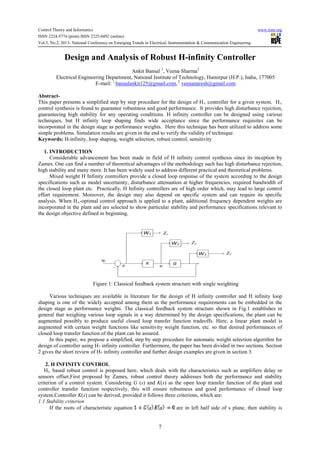
Control Theory and Informatics www.iiste.org
ISSN 2224-5774 (print) ISSN 2225-0492 (online)
Vol.3, No.2, 2013- National Conference on Emerging Trends in Electrical, Instrumentation & Communication Engineering
7
Design and Analysis of Robust H-infinity Controller
Ankit Bansal 1
, Veena Sharma2
Electrical Engineering Department, National Institute of Technology, Hamirpur (H.P.), India, 177005
E-mail: 1
bansalankit125@gmail.com, 2
veenanaresh@gmail.com
Abstract-
This paper presents a simplified step by step procedure for the design of H∞ controller for a given system. H∞
control synthesis is found to guarantee robustness and good performance. It provides high disturbance rejection,
guaranteeing high stability for any operating conditions. H infinity controller can be designed using various
techniques, but H infinity loop shaping finds wide acceptance since the performance requisites can be
incorporated in the design stage as performance weights. Here this technique has been utilized to address some
simple problems. Simulation results are given in the end to verify the validity of technique.
Keywords: H-infinity, loop shaping, weight selection, robust control, sensitivity
1. INTRODUCTION
Considerable advancement has been made in field of H infinity control synthesis since its inception by
Zames. One can find a number of theoretical advantages of the methodology such has high disturbance rejection,
high stability and many more. It has been widely used to address different practical and theoretical problems.
Mixed weight H Infinity controllers provide a closed loop response of the system according to the design
specifications such as model uncertainty, disturbance attenuation at higher frequencies, required bandwidth of
the closed loop plant etc. Practically, H Infinity controllers are of high order which, may lead to large control
effort requirement. Moreover, the design may also depend on specific system and can require its specific
analysis. When H∞-optimal control approach is applied to a plant, additional frequency dependent weights are
incorporated in the plant and are selected to show particular stability and performance specifications relevant to
the design objective defined in beginning.
Figure 1: Classical feedback system structure with single weighting
Various techniques are available in literature for the design of H infinity controller and H infinity loop
shaping is one of the widely accepted among them as the performance requirements can be embedded in the
design stage as performance weights. The classical feedback system structure shown in Fig.1 establishes in
general that weighing various loop signals in a way determined by the design specifications, the plant can be
augmented possibly to produce useful closed loop transfer function tradeoffs. Here, a linear plant model is
augmented with certain weight functions like sensitivity weight function, etc. so that desired performances of
closed loop transfer function of the plant can be assured.
In this paper, we propose a simplified, step by step procedure for automatic weight selection algorithm for
design of controller using H- infinity controller. Furthermore, the paper has been divided in two sections. Section
2 gives the short review of H- infinity controller and further design examples are given in section 3.
2. H INFINITY CONTROL
H∞ based robust control is proposed here, which deals with the characteristics such as amplifiers delay or
sensors offset.First proposed by Zames, robust control theory addresses both the performance and stability
criterion of a control system. Considering G (s) and K(s) as the open loop transfer function of the plant and
controller transfer function respectively, this will ensure robustness and good performance of closed loop
system.Controller K(s) can be derived, provided it follows three criterions, which are:
1.1 Stability criterion
If the roots of characteristic equation are in left half side of s plane, then stability is

8
ensured.
1.2Performance Criterion
It establishes that the sensitivity is small for all frequencies where disturbances
and set point changes are large.
1.3Robustness criterion
It states that stability and performance should be maintained not only for the nominal model but also for a
set of neighboring plant models that result from unavoidable presence of modeling errors. Robust controllers
are designed to ensure high robustness of linear systems.
Guangzhong Cao, Suxiang Fan, Gang Xu, Arredondo and J. Jugo, ZdzislawGosiewski,
ArkadiuszMystokowski, proposed the detailed design procedure for control of linear system. Generally, the
norm of a transfer function, F, is its maximum value over the complete spectrum, and is represented as
=sup (1)
Here, is the largest singular value of a transfer function. The aim here is synthesize a controller which will
ensure that the H∞ norm of the plant transfer function is bounded within limits. Various techniques are there for
the design of the controllers such as two transfer function method and three transfer function method. The
former one has less computational complexities and so can be preferred over the former one for H∞ controller
synthesis. The formulation of robust control problem is depicted in Fig. 2. Here, ‘w’ is the vector of all
disturbance signals; ‘z’ is the cost signal consisting of all errors. ‘v’ is the vector consisting of measurement
variables and ‘u’ is the vector of all control variables.
Figure 2: Robust Control Problem
Conventionally, H∞ controller synthesis employs two transfer functions which divide a complex control
problem into two separate sections, one dealing with stability, the other dealing with performance. The
sensitivity function, S, and the complementary sensitivity function, T, which is required for the controller
synthesis and are given in (2) and (3).
Sensitivity function is the ratio of output to the disturbance of a system and complementary sensitivity function
is the ratio of output to input of the system.
Now our objective is to find a controller K, which, based on the information in v, generates a control signal
u, which counteracts the influence of w on z, thereby minimizing the closed loop norm w to z. This can be done
by bounding the values of for performance for robustness. Minimizing the norm
(4)
Where,
(5)
and are the weight functions to be specified by the designer. As we know that the ultimate objective of the
robust control is to minimize the effect of disturbance on output, the sensitivity S and the complementary
function T are to be reduced. To achieve this it is enough to minimize the magnitude of and which can be
done so by making

9
is the performance weighting function which limits the magnitude of the sensitivity function and is
the robustness weighting function to limit the magnitude of the complementary sensitivity function Most widely
used technique for selecting the weight functions for the synthesis of the controller is loop shaping technique.
As it is already known that the robust controller is designedso as to make the norm of the plant to its
minimum and so achieve this condition three weight functions are added to the plant for loop shaping. Basically,
the weight functions arelead-lag compensators and can modify the frequency response of the system as desired.
To obtain the desired frequency response for the plant, loop shaping is employed with the weight functions.
There are various methods for loop shaping. The parameters of the weight functions are to be varied so as to get
the frequency response of the whole system within desired limits.The block diagram in Fig. 3 describes the
mixed Sensitivity problem.
Figure 3: Plant model for the synthesis of controller
Figure 4: General control problem
The generalized plant P(s) is given as,
1
2
3
0
(6 )
0
s s
k s
t
z W W G
z W w
z W G u
e I G
−   
   
    =       
   
−   
Considering the following state space realizations
s A B
G
C D
 
= 
 
,
s
s s
s
s s
A B
W
C D
 
= 
 
,
s
ks ks
ks
ks ks
A B
W
C D
 
= 
 
,
s
t t
t
t t
A B
W
C D
 
=  
 
’
a possible state space realization for P(s) can be written as

10
1 1
1 11 12
2 21 22
0
(7)
0
S S
KS
T
W W G
A B B
W
P C D D
W G
C D D
I G
− 
  
  = =   
    − 
From (6) and (7) we can write a mixed sensitivity problem as
(8)
s
ks
t
W S
P W KS
W T
 
 =  
  
In case of mixed sensitivity problem our objective is to find a rational function controller K(s) and to make the
closed loop system stable satisfying the following expression
min min (9)
s
ks
t
W S
P W KS
W T
 
 = = γ 
  
where, P is the transfer function from w to Z i.e
(10)zwT = γ
where, zwT P= is the cost function. Applying the minimum gain theorem, we can make the norm of
zwT less than unity, i.e,
min min 1 (11)
s
zw ks
t
W S
T W KS
W T
 
 = ≤
 
  
Therefore we can achieve a stabilizing controller K(s) is achieved by solving the algebraic Riccati
equations, thereby, minimizing the cost function γ.
As mentioned in the robust control theory the synthesis of the controller requires the selection of two
weight functions. There are various methods available in literature for selection of weights. In most of these
design methods the weighting functions are selected using trial and error and further the H∞ controller is
synthesized by loop shaping technique. But train and error procedure may not end up in a stabilizing controller
and thisis the main draw back in this type of synthesis.
The weights , and are the tuning parameters and it typically requires some iterations to obtain
weights which will yield a good controller. That being said, a good starting point is to choose
0
0
/
(12)s
s M
W
s A
+ ω
=
+ ω
. (13)ksW const=
0
0
/
(14)t
s M
W
As
+ ω
=
+ ω
where A < 1 is the maximum allowed steady state offset, is the desired bandwidth and M is the sensitivity
peak (typically A = 0.01 and M = 2). For the controller synthesis, the inverse of is an upper bound on the
desired sensitivity loop shape, and will effectively limit the controller output u which is symmetric to
around the line .Fig shows the two weighting functions for the parameter values A = 0.01(= −40dB), M
= 2(= 6dB) and rad/sec.
3. DESIGN EXAMPLE
3.1 Example 1
Let the plant and nominal model are considered as follows:

11
Plant =
( )( )
2
85
1 0.1 2s s+ +
The weighting functions designed by the algorithm are serves to satisfy the control specification for the
sensitivity characteristic and the response characteristic.Here it can be taken as
5
5 4
s
s
W
s e
+
=
+ −
and
1;ksW =
This produces the following controller
( )
6 5 4 3 2
8 7 6 5 4 3 2
4976 4.08 005 1.274007 1.835 008 1.127 009 1.752 009 7.917 008 3.981 005
6827 7.039 005 3.094 007 6.211 008 4.799 009 4.212 009 4.209 006 1060
e s s e s e s e s e s e
K S
s s e s e s e s e s e s e s
+ + + + + + +
=
+ + + + + + + +
With GAMMA=1.2441
The largest singular value Bode plots of the closed-loopsystem are shown in Fig. 5. We note that the
controller typically gives arelatively at frequency response since it tries to minimize the peak of the
frequencyresponse.
10
-2
10
-1
10
0
10
1
10
2
10
3
10
4
1.05
1.1
1.15
1.2
1.25
Frequency [rad/sec]
Amplitude
Figure 5:The largest singular value plot of the closed-loop
System with a controller
10
-2
10
-1
10
0
10
1
10
2
10
3
10
10
-10
10
-8
10
-6
10
-4
10
-2
10
0
10
2
10
4
Frequency [rad/sec]
Amplitude
Figure 6:The frequency responses of S,T,KS and
GKwith K
Robust H∞ controller developed not only operates on the known plant in a stable environment, but alsoprovides
good control for a set of nearby uncertain plants.The system must be robust enough to providegood performance
and stability over the uncertainty. Singular values are a good measure of the systemrobustness. The Fig.6 plots
the singular value plot of the system with H infinity control.

12
0 0.1 0.2 0.3 0.4 0.5 0.6 0.7 0.8 0.9 1
0
0.2
0.4
0.6
0.8
1
0 0.1 0.2 0.3 0.4 0.5 0.6 0.7 0.8 0.9 1
0
0.5
1
Amplitude
time
Figure 7: Step response
3.2 Example 2
The given plant model is,
Plant = 2
39
25 7 4 005s s e+ −
with the weight function as,
( )
300
3 15
s
W s
s
+
=
+
( )
100
200
s
W t
s
+
=
+
Solving with the help of weight functions, we get the controller as,
( )
3 2
4 3 2
1.385 015 5.016 017 5.118 019 1.25 021
7.537 006 2.243 011 6.926 014 3.457 015
e s e s e s e
K s
s e s e s e s e
+ + +
=
+ + + +
With GAMMA=0.7785
10
-2
10
-1
10
0
10
1
10
2
10
3
10
4
0.755
0.76
0.765
0.77
0.775
0.78
0.785
Frequency [rad/sec]
Amplitude
Figure 8: The largest singular value plot of the closed-loop
System with a controller
The largest singular value Bode plots of the closed-loopsystem are shown in Figure 8. We note that the
controller typically gives arelatively at frequency response since it tries to minimize the peak of the
frequencyresponse.
10
-2
10
0
10
2
10
4
10
6
10
-4
10
-2
10
0
10
2
Frequency [rad/sec]
Amplitude
Figure 9: The frequency responses of S, T, and
GK with K

13
Robust H∞ controller developed not only operates on the known plant in a stable environment, but alsoprovides
good control for a set of nearby uncertain plants.The system must be robust enough to providegood performance
and stability over the uncertainty. Singular values are a good measure of the system robustness. The Fig (9) plots
the singular value plot of the system with H infinity control.
0 0.1 0.2 0.3 0.4 0.5 0.6 0.7 0.8 0.9 1
-0.5
0
0.5
1
0 0.1 0.2 0.3 0.4 0.5 0.6 0.7 0.8 0.9 1
0
0.5
1
1.5
Amplitude
time
Figure 10: Step response
4. CONCLUSION
A step-wise procedurefor the design of H∞ controller has been presented in detail in this paper. It has been
observed from analysis that H∞ controller guarantees robustness, good performance in terms of sensitivity and
provides high disturbance rejection, providing high stability for any operating conditions. Simple illustrative
examples have been considered and loop shaping technique has been utilized to solve the problems. Simulation
results presentedhere verify the validity of loop shaping technique.
5. REFERENCES
[1]. Zames G., "Feedback of Optimal Sensitivity: Model Reference Transformations, Multiplicative Semi-
norms, and Approximate Inverses", IEEETrans. AC, Vol. AC-26, 1981, pp301-320.
[2]. Limbeer, D.J.N. and Kasenally, E., 1986, "H∞Optimal Control of a Synchronous Turbogenerator" in
Proc. IEEE 25th Conf. Decision Contr. (Athens, Greece), Dec. 1986, pp 62-65.
[3]. Doyle J. C., Glover K., Khargonekar P. P. and Francis B. A., State- Space Solutions to Standard H2and
,control problems, Proc. 1988 American Control Conference, Atlanta (1988).
[4]. Glover K. and Doyle J.C., State-Space Formulae for all Stabilizing Controllers that Satisfy an - Norm
Bound and Relations to Risk Sensitivity, Systems and Control Letters 11, 167/172 (1988).
[5]. Guangzhong Cao, Suxiang Fan, Gang Xu “The Characteristics Analysis of Magnetic Bearing Basedon
H-infinity Controller”,Proceedings of the 51th World Congress on Intelligent Control and Automation,
June 15-19, 2004, Hangzhou, P.R. China.
[6]. Arredondo and J. Jugo, “Active Magnetic Bearings Robust Control Design based on Symmetry
Properties”, Proceedings of the American Control Conference,USA, July 11-13, 2007
[7]. Beaven R.W., Wright M.T. and Seaward D.R., “Weighting function selection in the H∞ design
Process”, Control Eng. Practice, Vol.4, No. 5, pp. 625-633, 1996
[8]. Jiankun Hu, Christian Bohn, Wu H.R., “Systematic H∞ weighting function selection and its application
to the real-time control of a vertical take-off aircraft”, Control Engineering Practice 8 (2000) 241-252
[9]. Carl R. Knospe, “Active magnetic bearings for machining applications, Control Engineering Practice
15 (2007) 307–313
[10]. Mark Siebert, Ben Ebihara,Ralph Jansen, Robert L. Fusaro and Wilfredo Morales, Albert Kascak,
Andrew Kenny, “A Passive Magnetic Bearing Flywheel”, NASA/TM—2002-211159, 36th Intersociety
Energy Conversion Engineering Conference cosponsored by the ASME, IEEE, AIChE, ANS, SAE, and
AIAA Savannah, Georgia, July 29–August 2, 2001,
[11]. Verde C. and Flores J., “Nominal model selection for robust control design”, proceedings of the
American control conference, seatle, Washington, 1996.
[12]. Beaven W., Wright M.T. and Seaward D.R., “Weighting Function selection in the H∞ design process”,
control eng. practice, vol. 4, no. 5, pp. 625-633, 1996
[13]. Engell S., “Design of robust control systems with time-domain specifications”, control eng. practice,

14
vol. 3, no. 3, pp. 365-372, 1995
[14]. DidierhEnrion, Michael Sebek and Sophie Tarbouriech, “Algebraic approach to robust controller design:
A geometric interpretation”, Proceedings of the American control conference,philadelphia,
pennsylvaniajune, 1998
[15]. Jiang Z. F., Wu H. C., Lu H., Li C. R., “Study on the Controllability for Active Magnetic Bearings”,
Journal of Physics: Conference Series13 (2005) 406–409
[16]. Hochschulverlag A.G., Kokame H., Kobayashi H., Mori T., Robust performance for linear delay-
differential systems with time-varying uncertainties, IEEE Trans. on Automatic Control, Vol.43, No.2,
223-226, 1998.
[17]. Euu T. J., Tong H. K., Hong B. P., H-infinityoutput feedback controller design for linear systems with
time-varying delayed state, IEEE Trans. on Automatic Control, Vol.43, No.7, 971-974, 1998.
[18]. Lee J. H., Lim S. W., Kwon W. H., Memoryless controllers for state delayed systems, IEEE Trans.
on Automatic Control, Vol.39, No.1, 159-162, 1994.
[19]. Liu H. X., Xu B. G., Zhu X. F., Tang S. T., LMI Approach of dynamic output feedback control for
large-scale interconnected time-delay systems, Journal of South China University of Technology,
Vol.29, No.11, 37-41, 2001.
[20]. Doyle J. C., Lecture Notes, in Adaances in Multivariable Control, ONR/Honeywell Workshop,
Minneapolis (1984)
[21]. Francis B. A., ACourse in , control Theory, Springer-Verlag (1987)
[22]. Kimura H. and Kawatani R., Synthesis ofH, Controllers Based on Conjugation, Proc.of CDC, 7/13
(1988)
[23]. Zhou K. and Khargonekar P. P., An Algebraic Riccati Equation Approach to , Optimization, Systems
and Control Letters 11, 85/91 (1988)
[24]. Sampei M., Mita T., Chida Y and Nakamichi M., A Direct Approach To Control Problems Using
Bounded Real Lemma, Conference on Decision and Control, Florida (1989)
[25]. Nair S. Sarath, Automatic weight Selection Algorithm for Designing H-Infinity controller for Active
Magnetic Bearing, International Journal of Science and Technology (IJEST), Vol. 3, No. 1, Jan 2011.
[26]. Hvostov S. Harry, Simplifying H-Infinity Controller Synthesis via Classical feedback System Structure,
Proceeding of the 28th
Conference on Decision and Control, Tampa, Florida, Dec,1989

This academic article was published by The International Institute for Science,
Technology and Education (IISTE). The IISTE is a pioneer in the Open Access
Publishing service based in the U.S. and Europe. The aim of the institute is
Accelerating Global Knowledge Sharing.
More information about the publisher can be found in the IISTE’s homepage:
http://www.iiste.org
CALL FOR PAPERS
The IISTE is currently hosting more than 30 peer-reviewed academic journals and
collaborating with academic institutions around the world. There’s no deadline for
submission. Prospective authors of IISTE journals can find the submission
instruction on the following page: http://www.iiste.org/Journals/
The IISTE editorial team promises to the review and publish all the qualified
submissions in a fast manner. All the journals articles are available online to the
readers all over the world without financial, legal, or technical barriers other than
those inseparable from gaining access to the internet itself. Printed version of the
journals is also available upon request of readers and authors.
IISTE Knowledge Sharing Partners
EBSCO, Index Copernicus, Ulrich's Periodicals Directory, JournalTOCS, PKP Open
Archives Harvester, Bielefeld Academic Search Engine, Elektronische
Zeitschriftenbibliothek EZB, Open J-Gate, OCLC WorldCat, Universe Digtial
Library , NewJour, Google Scholar

Design and analysis of robust h infinity controller

Recommended

Recommended

More Related Content

What's hot

What's hot (20)

Viewers also liked

Viewers also liked (7)

Similar to Design and analysis of robust h infinity controller

Similar to Design and analysis of robust h infinity controller (20)

More from Alexander Decker

More from Alexander Decker (20)

Recently uploaded

Recently uploaded (20)

Design and analysis of robust h infinity controller