SlideShare a Scribd company logo
1 of 32
Download to read offline
Elementary Discussions on Group Theory:
A Physicists’ Point of View
Calcutta University PG-I and PG-II
Anirban Kundu
Contents
1 Why Should We Study Group Theory? 3
2 What is a Group? 3
3 Discrete and Finite Groups 5
3.1 Multiplication Table . . . . . . . . . . . . . . . . . . . . . . . . . . . . . . . 5
3.2 Isomorphism and Homomorphism . . . . . . . . . . . . . . . . . . . . . . . . 6
3.3 Conjugacy Classes . . . . . . . . . . . . . . . . . . . . . . . . . . . . . . . . 6
4 Representation of a Group 7
4.1 Reducible and Irreducible Representations . . . . . . . . . . . . . . . . . . . 9
4.2 Schur’s Lemma and the Great Orthogonality Theorem . . . . . . . . . . . . 9
5 Lie Groups and Lie Algebras 11
5.1 Algebra of Generators . . . . . . . . . . . . . . . . . . . . . . . . . . . . . . 12
6 SU(2) 15
6.1 Product Representation of SU(2) . . . . . . . . . . . . . . . . . . . . . . . . 18
6.2 Weight and Root: A Pictorial Way of Composition . . . . . . . . . . . . . . 19
6.3 SU(2) and SO(3) . . . . . . . . . . . . . . . . . . . . . . . . . . . . . . . . . 21
6.4 Guiding Principle to Write the Lagrangian . . . . . . . . . . . . . . . . . . . 21
7 SU(3) 22
7.1 Example: Quark Model and the Eightfold Way . . . . . . . . . . . . . . . . . 23
7.2 The Method of Young Tableaux . . . . . . . . . . . . . . . . . . . . . . . . . 25
8 Lorentz Group 29
8.1 More about Lorentz Groups . . . . . . . . . . . . . . . . . . . . . . . . . . . 30
8.2 The Inhomogeneous Lorentz Group . . . . . . . . . . . . . . . . . . . . . . . 31
9 Epilogue 32
This note is based upon the following excellent textbooks:
Tinkham: Group Theory & Quantum Mechanics
Joshi: Elements of Group Theory for Physicists
Georgi: Lie Groups in Particle Physics
Cheng and Li: Gauge Theory of Elementary Particle Physics
Tung: Group Theory in Physics
Schweber: Relativistic Quantum Field Theory
You are always advised to read the original textbooks. Remember that the supplementary
problems form an integral part of the course.
Caveat Emptor: This note emerged from the lectures I have delivered over the last few years.
The coverage is far from exhaustive. In fact, there are a number of important topics (e.g., rotation
group) that I generally do not have time to touch in the class, and have incorporated here only
briefly. Maybe I will try to do full justice to them later. The language may not be as clear as I
have planned. I will be extremely glad to have suggestions. The figures have been drawn with the
software xfig, and I have not given too much time for a flawless job there. Be careful!
2
1 Why Should We Study Group Theory?
Group theory can be developed, and was developed, as an abstract mathematical topic.
However, we are not mathematicians. We plan to use group theory only as much as is needed
for physics purpose. For this, we focus more on physics aspects than on mathematical rigour.
All complicated proofs have been carefully avoided, but you should consult the reference
books if you are interested.
Almost every time, we have to use some symmetry property of the system under study to
get more information (like the equations of motion, or the energy eigenfunctions) about it.
For example, if the potential in the Schr¨odinger equation is symmetric under the exchange
x → −x (this is known as a parity transformation), even without solving, we can say that
the wavefunctions are bound to have a definite parity. Group theory is nothing but a mathe-
matical way to study such symmetries. The symmetry can be discrete (e.g., reflection about
some axis) or continuous (e.g., rotation). Thus, we need to study both discrete and contin-
uous groups. The former is used more in solid state physics, particularly in crystallographic
studies, while the latter is used exhaustively in quantum mechanics, quantum field theory,
and nuclear and particle physics.
2 What is a Group?
A group G is a set of discrete elements a, b, · · · x alongwith a group operator 1
, which we will
denote by ⊙, with the following properties:
• Closure: For any two elements a, b in G, a ⊙ b must also be in G. We will try to
avoid the mathematical symbols as far as practicable, but let me tell you that in some
texts this is written as ∀a, b ∈ G, a ⊙ b ∈ G. The symbol ∀ is a shorthand for “for
all”. Another commonly used symbol is ∃: ∃a ∈ G means “there exists an a in G such
that”.
• Associativity: For any three elements a, b, c in G,
a ⊙ (b ⊙ c) = (a ⊙ b) ⊙ c, (1)
i.e., the order of the operation is not important.
• Identity: The set must contain an identity element e for which a ⊙ e = e ⊙ a = a.
• Inverse: For every a in G, there must be an element b ≡ a−1
in G so that b⊙a = a⊙b = e
(we do not distinguish between left and right inverses). The inverse of any element a
is unique; prove it.
These are essential properties of a group. Furthermore, if a ⊙ b = b ⊙ a, the group is said
to be abelian. If not, the group is non-abelian. Note that no two elements of a group are
identical. If the number of group elements (this is also called the order of the group) is finite,
it is a finite group; otherwise it is an infinite group. Elements of a finite group are necessarily
1
In most of the texts this is called group multiplication or simply multiplication operator. Let me warn you
that the operator can very well be something completely different from ordinary or matrix multiplication.
For example, it can be addition for the group of all integers.
3
discrete (finite number of elements between any two elements). An infinite group may have
discrete or continuous elements.
Now some examples:
• The additive group of all integers. It is an abelian infinite group. The group operation
is addition, the identity is 0, and the inverse of a is just −a. Note that the set of all
positive integers is not a group; there is no identity or inverse.
• The multiplicative group of all real numbers excluding zero (why?).
• Zn, the multiplicative group of n-th roots of unity (this is also called the cyclic group
of order n). For example, Z3 = {1, ω, ω2
} where ω = 11/3
; Z4 = {1, i, −1, −i}. The
operation is multiplication and the identity is 1 (what is the inverse?).
• The n-object permutation group Sn. Consider a 3-element permutation group S3 =
{a, b, c}. There are six elements: P0, which is the identity and does not change the
position of the elements; P12, which interchanges positions 1 and 2, i.e., P12 → (b, a, c).
Similarly, there are P13 and P23. Finally, there are P123 and P132, with
P123(a, b, c) → (c, a, b)
P132(a, b, c) → (b, c, a), (2)
i.e., P123 takes element of position 1 to position 2, that of position 2 to position 3 and
that of position 3 to position 1. Obviously, P123 = P231 = P312, and similarly for P132.
• C4v, the symmetry group of a square. Consider a square in the x-y plane with corners
at (a, a), (a, −a), (−a, −a), and (−a, a). The symmetry operations are rotations about
the z axis by angles π/2, π and 3π/2 (generally, they are taken to be anticlockwise,
but one can take clockwise rotations too), reflections about x and y axes, and about
the diagonals.
• U(n), the group of all n × n unitary matrices. Thus, the elements of U(1) are pure
phases like exp(iθ). It is the group of phase transformations. Apart from U(1), all
U(n)s are non-abelian. When we say that an individual phase in the wave function
does not have any physical significance, we mean that the Lagrangian is so constructed
that it is invariant under a U(1) transformation ψ → eiθ
ψ.
• SU(n), the group of all n × n unitary matrices with determinant unity (also called
unitary unimodular matrices). This is the most important group in particle physics.
All SU groups are non-abelian, of which the simplest is SU(2). The simplest member
of SU(2) is the two-dimensional rotation matrix
cos θ sin θ
− sin θ cos θ
, characterised by
different values of θ. Check that the matrix
eiα
cos θ eiβ
sin θ
−e−iβ
sin θ e−iα
cos θ
is also a member
of SU(2).
• O(n), the group of all n × n orthogonal matrices. It is non-abelian for n ≥ 2.
• SO(n), the group of all n×n orthogonal matrices with determinant unity. Thus, SO(3)
is the familiar rotation group in three dimensions. The S in SU(n) and SO(n) stands
for special, viz., the unimodularity property.
4
The first group is infinite but discrete, i.e., there are only a finite number of group
elements between any two elements of the group. The second group is infinite and continuous,
since there are infinite number of reals between any two real numbers, however close they
might be. Zn and Sn are obviously discrete, since they are finite. The last four groups are
infinite and continuous, which means that there are an infinite number of group elements
between two given elements of the group. We will be interested in only those continuous
groups whose elements can be parametrised by a finite number of parameters. Later, we will
see that this number is equal to the number of generators of the group.
Q. Show that the number of independent elements of an N × N unitary matrix is N2
, and
that of an N × N unimodular matrix is N2
− 1. [Hint: U†
U = 1, so det U det U†
= 1, or
|det U|2
= 1, so that the determinant must have modulus unity and a form like exp(iθ).]
Q. Show that the determinant of a 2 × 2 orthogonal matrix must be either +1 or −1. [Hint:
Write the matrix as
a b
c d
and construct the constraint equations. Show that this leads to
(ad − bc)2
= 1.]
3 Discrete and Finite Groups
3.1 Multiplication Table
A multiplication table is nothing but a compact way to show the results of all possible
compositions among the group elements. Obviously, this makes sense only for finite groups.
For example, the multiplication tables for Z4 and S3 are, respectively,
1 i −1 −i
1 1 i −1 −i
i i −1 −i 1
−1 −1 −i 1 i
−i −i 1 i −1
P0 P12 P13 P23 P123 P132
P0 P0 P12 P13 P23 P123 P132
P12 P12 P0 P132 P123 P23 P13
P13 P13 P123 P0 P132 P12 P23
P23 P23 P132 P123 P0 P13 P12
P123 P123 P13 P23 P12 P132 P0
P132 P132 P23 P12 P13 P0 P123
One should note a few things. First, Z4 is obviously abelian, and hence the multiplication
table is symmetric, but S3 is non-abelian (e.g., P13P23 = P23P13). For both of them, all ele-
ments occur only once in each row or column. This is a general property of the multiplication
table and is easy to prove. Suppose two elements a ⊙ b and a ⊙ c are same. Multiply by
a−1
, so b = c, contrary to our assumption of all elements being distinct. However, number
of elements in each row or column is equal to the order of the group, so all elements must
occur once and only once.
5
3.2 Isomorphism and Homomorphism
Consider the symmetry group of an equilateral triangle, with six elements (identity, three
reflections about the medians, and rotations by 2π/3 and 4π/3). The multiplication table
is identical with S3. Only this (not just the number of elements) shows that the groups
behave in an identical way. This is known as isomorphism: we say that these two groups are
isomorphic to one another. Thus, isomorphism means a one-to-one correspondence between
the elements of two groups so that if a, b, c ∈ G and d, e, f ∈ H, and a, b, c are isomorphic to
d, e, f respectively, then a ⊙ b = c implies d ⊙ e = f, for all a, b, c and d, e, f. Note that e is
just an element of H, not the identity; also, the operations in G and H may be completely
different. Try to convince yourself that the identity of one group must be mapped on to the
identity of the second group.
Thus, S3 is isomorphic to C3. If we consider only rotational symmetries, then the three-
member subgroup (a subset of a group that itself behaves likes a group) of C3 is isomorphic
to Z3. In fact, this is a general property: the rotational symmetry group of any symmetric
n-sided polygon, having 2π/n rotation as a symmetry operation, is isomorphic to Zn. Check
this for Z4. This cannot be a coincidence; what is the physical reason behind this?
If the mapping is not one-to-one but many-to-one, the groups are said to be homomorphic
to one another. Obviously, in a many-to-one mapping, some information is lost. All groups
are homomorphic to the group containing the identity; but that is a very bad mapping,
since no information about the group structure is retained. A better homomorphism occurs
between Z2 and Z4, where (1, −1) of Z4 is mapped to 1 of Z2, and (i, −i) of Z4 is mapped
to −1 of Z2. Isomorphism is only a special case of homomorphism, but in general, the two
groups which are homomorphic to one another should be of different order, and the ratio
of their orders n/m should be an integer k. In this case, set of k elements of G is mapped
to one element of H. The set containing identity in G must be mapped to the identity of
H: prove this. Also prove that this set itself must form a group. Such a group, which is
completely embedded in a bigger group, is known as a subgroup. Every group has two trivial
subgroups: the identity and the entire group!
3.3 Conjugacy Classes
Consider a group G with elements {a, b, c, d, · · ·}. If aba−1
= c, (from now on we drop the ⊙
symbol for group operation), then b and c are said to be conjugate elements. If b is conjugate
to both c and d, then c and d are conjugate to each other. The proof goes like this: Suppose
aba−1
= c and hbh−1
= d, then b = a−1
ca and hence ha−1
cah−1
= d. But ah−1
is a member
of the group, and hence its inverse, ha−1
, too (why the inverse of ah−1
is not a−1
h?). So c
and d are conjugate to each other.
It is trivial to show that the identity element in any group is conjugate only to itself, and
for an abelian group all members are conjugate to themselves only.
Now, any discrete group can be separated into sets of elements (need not having the same
number of elements) where all members of a set are conjugate to each other but no member
of any set is conjugate to another member of a different set. In that case, the sets are called
conjugacy classes or simply classes.
Let us take C4v, the symmetry group of a square. The symmetry operations are 1
(identity), rπ/2, rπ, r3π/2 (rotations, may be clockwise or anticlockwise), Rx, Ry (reflections
6
about x and y axes, passing through the centre of the square), and RNE and RSE, the
reflections about the NE and the SE diagonal. [In some texts you will see different notations,
but these are equally good, if not more transparent.]
These eight elements form a group; that can be checked from the multiplication table.
The group is non-abelian. However, the first four members form an abelian group isomorphic
to Z4. The eight elements can be divided into five classes: (1), (rπ), (rπ/2, r3π/2), (Rx, Ry),
(RNE, RSE). It is left as an exercise to check the class structure.
What is the physical significance of classes? In other words, can we guess which elements
should be in a particular class? The answer is yes: note that the conjugacy operation is
nothing but a similarity transformation performed with the group elements. This will be
more obvious in the next section when we show how to represent the abstract group elements
with matrices, in particular unitary matrices.
Identity must be a class by itself. rπ/2 and r3π/2 belong to the same class because there
is an element of the group which relates rotation by π/2 with rotation by 3π/2: just the
reflection about the x or y axis, which makes a clockwise rotation anticlockwise and vice
versa. Similarly, Rx and Ry belong to the same class since there is an operation that relates
them: rotation by π/2. However, Rx and RNE cannot belong to the same class, since there
is no symmetry operation of rπ/4.
4 Representation of a Group
The permutation group discussed above is an example of a transformation group on a physical
system. In quantum mechanics, a transformation of the system is associated with a unitary
operator in the Hilbert space (time reversal is the only example of antiunitary transformation
that is relevant to us). Thus, a transformation group of a quantum mechanical system is
associated with a mapping of the group to a set of unitary operators 2
. Thus, for each a
in G there is a unitary operator D(a). Furthermore, this mapping must preserve the group
operation, i.e.,
D(a)D(b) = D(a ⊙ b) (3)
for all a and b in G. A mapping which satisfies eq. (3) is called a representation of the group
G. In fact, a representation can involve nonunitary operators so long as they satisfy eq. (3).
For example, the mapping
D(n) = exp(inθ) (4)
is a representation of the additive group of integers, since
exp(imθ) exp(inθ) = exp(i(n + m)θ). (5)
Check that the following mapping is a representation of the 3-element permutation group
S3:
D(1) =



1 0 0
0 1 0
0 0 1


 ; D(12) =



0 1 0
1 0 0
0 0 1


 ; D(13) =



0 0 1
0 1 0
1 0 0


 ;
2
If this mapping is one-to-one, the representation is called faithful. We will deal with faithful representa-
tions only.
7
D(23) =



1 0 0
0 0 1
0 1 0


 ; D(123) =



0 0 1
1 0 0
0 1 0


 ; D(321) =



0 1 0
0 0 1
1 0 0


 . (6)
Particularly, check the multiplication table.
In short, a representation is a specific realisation of the group operation law by finite or
infinite dimensional matrices. For abelian groups, their representative matrices commute.
Consider a n-dimensional Hilbert space. Thus, there are n orthonormal basis vectors. Let
|i be a normalised basis vector. We define the ij-th element of any representation matrix
D(a) as
[D(a)]ij = i|D(a)|j , (7)
so that
D(a)|i =
j
|j j|D(a)|i =
j
[D(a)]ji|j . (8)
From now on, we will freely translate from one language (representations as abstract linear
operators) to the other (representations as matrices). Anyway, it is clear that the dimension
of the representation matrices is the same as that of the Hilbert space.
Thus, the elements of a group can be represented by matrices. The dimension of the
matrices has nothing to do with the order of the group. But the matrices should be all
different, and there should be a one-to-one mapping between the group elements and the
matrices; that’s what we call a faithful representation. Obviously, the representative matrices
are square, because matrix multiplication is defined both for D(a)D(b) and D(b)D(a). The
representation of identity must be the unit matrix, and if T(a) is the representation of a,
then T−1
(a) = T(a−1
) is the representation of a−1
. The matrices must be non-singular; the
inverse exists.
However, the matrices need not be unitary. But in quantum mechanics we will be con-
cerned with unitary operators, and so it is better to show now that any representation of a
group is equivalent to a representation by unitary matrices. Two representations D1 and D2
are equivalent if they are related by a similarity transformation
D2(a) = SD1(a)S−1
(9)
with a fixed operator S for all a in the group G.
Suppose T(a) is the representation of a group G. T(a)s need not be unitary. Define a
hermitian matrix
H =
a∈G
T(a)T†
(a). (10)
This matrix, being hermitian, can be diagonalised by a unitary transformation. Let U†
HU =
Hd. Hd is a real diagonal matrix whose elements are the eigenvalues of H. Using the form
of H,
Hd = U†
a∈G
T(a)T†
(a)U =
a∈G
U†
T(a)U U†
T†
(a)U =
a∈G
T (a)T †
(a) (11)
where T (a) is also a representation (remember U†
= U−1
). Take the k-th diagonal element
of Hd:
[Hd]kk ≡ dk =
a∈G j
Tkj(a)T †
jk(a) =
a∈G j
|Tkj(a)|2
. (12)
8
Thus dk ≥ 0. The case dk = 0 can be ruled out since in that case a particular row in all the
representative matrices is zero and the determinants are zero, so all matrices are singular.
So dk is positive for all k, and we can define a diagonal matrix H
1/2
d whose k-th element is
√
dk. Construct the matrix V = UH
1/2
d and the representation Γ(a) = V −1
T(a)V . We now
show that all Γ matrices are unitary, completing the proof.
We have Γ(a) = V −1
T(a)V = H
−1/2
d U−1
T(a)UH
1/2
d = H
−1/2
d T (a)H
1/2
d , and
Γ(a)Γ†
(a) = H
−1/2
d T (a)H
1/2
d H
1/2
d T †
(a)H
−1/2
d
= H
−1/2
d T (a)HdT †
(a)H
−1/2
d
= H
−1/2
d T (a)
b∈G
T (b)T †
(b)T †
(a)H
−1/2
d
= H
−1/2
d
b∈G
T (ab)T †
(ab)H
−1/2
d
= H
−1/2
d HdH
−1/2
d = 1. (13)
Here we have used the rearrangement theorem: as long as we sum over all the elements of
the group, how we denote them is immaterial.
This theorem depends on the convergence of a number of sums. For an infinite group,
this is not so straightforward. However, for Lie groups (to be discussed in the next section)
this theorem holds.
4.1 Reducible and Irreducible Representations
A representation D is reducible if it is equivalent to a representation D′
with block-diagonal
form (or itself block-diagonal):
D′
(x) = SD(x)S−1
=
D′
1(x) 0
0 D′
2(x)
. (14)
The vector space on which D′
acts breaks up into two orthogonal subspaces, each of which is
mapped into itself by all the operators D′
(x). The representation D′
is said to be the direct
sum of D′
1 and D′
2:
D′
= D′
1 ⊕ D′
2. (15)
A representation is irreducible if it cannot be put into block-diagonal form by a similarity
transformation.
4.2 Schur’s Lemma and the Great Orthogonality Theorem
Before closing the section on discrete groups, we will prove a very important theorem on the
orthogonality of different representations of a group. This theorem tells you that if you have
two different representations of a group which are both irreducible but inequivalent to each
other, then the ‘dot product’ of these two representations is zero. What is a ‘dot product’?
Each of these representations form a g-dimensional vector space, where g is the order of
the group. The ‘dot product’ is something like taking a matrix from one space, taking its
corresponding matrix from the other space, taking any two elements of these matrices, and
9
then sum over all elements of the group. A more mathematical definition will soon follow,
but before that we need to prove two lemmas by Schur.
Schur’s Lemma 1. If a matrix P commutes with all representative matrices of an irre-
ducible representation, then P = c1, a multiple of the unit matrix.
Proof. Given, PT(a) = T(a)P for all a ∈ G, where we take T(a)s to be a unitary
representation without loss of generality. Suppose the dimension of T(a) is n × n; evidently,
that should be the dimension of P. T(a)s possess a complete set of n eigenvectors. So does
P, since [P, T(a)] = 0. Let ψj be some eigenvector of P with eigenvalue cj: Pψj = cjψj.
Then PT(a)ψj = cjT(a)ψj. So both ψj = T(1)ψj and T(a)ψj, two independent eigenvectors,
have same eigenvalue. How many such degenerate states exist? Obviously n, since if the
number of such degenerate states be m < n, we have an m-dimensional invariant subspace
in the whole n-dimensional vector space, so the original space is not irreducible. Thus, all
cjs are equal, and P = c1.
Schur’s Lemma 2. Suppose you have two irreducible representations Ti
(a) and Tj
(a) of
dimension li and lj respectively. If a matrix M satisfies Ti
(a)M = MTj
(a) for all a ∈ G,
then either (i) M = 0, a null matrix, or (ii) det M = 0, in which case Ti
and Tj
are equivalent
representations.
Proof. The dimension of M is li × lj. If li = lj, M is a square matrix. If its determinant
is not zero, Ti
and Tj
are obviously equivalent representations.
First, we show, with the help of the first lemma, that M†
M is a multiple of the unit
matrix. Take the hermitian conjugate of both sides of the defining equation:
M†
Ti†
(a) = Tj†
(a)M†
⇒ M†
Ti
(a−1
) = Tj
(a−1
)M†
,
M†
Ti
(a−1
)M = Tj
(a−1
)M†
M ⇒ M†
MTj
(a−1
) = Tj
(a−1
)M†
M. (16)
This is true for all the elements of G, so M†
M = c1. If M is a square matrix and c = 0,
then the representations are equivalent. If c = 0, then
(M†
M)ii =
k
|Mki|2
= 0. (17)
This is true only if Mki = 0 for all k. But i is arbitrary and can run from 1 to n. So M = 0.
Now suppose li = lj. Let li < lj. Add lj −li rows of zero to M to get a square matrix M,
whose determinant is obviously zero. But M†
M = M†
M, and since the first one is zero, so
is the second one. Again take the (i, i)-th element of M†
M to get M = 0.
The Great Orthogonality Theorem says that if Ti
and Tj
are two inequivalent irre-
ducible representations of a group G, then
a∈G
Ti
km(a)Tj
ns(a−1
) =
g
li
δijδksδmn, (18)
where li and lj are the dimensions of the representations Ti
and Tj
respectively, and g is the
order of the group.
Proof. Consider a matrix M constructed as
M =
a∈G
Ti
(a)XTj
(a−1
) (19)
where X is an arbitrary matrix, independent of the group elements. Note that if the repre-
sentations are unitary then Tj
(a−1
) = Tj†
(a). Let Ti
and Tj
be two inequivalent irreducible
10
representations of dimensions li and lj respectively. Multiplying both sides of eq. (19) by
Ti
(b), where b ∈ G, we get
Ti
(b)M =
a∈G
Ti
(ba)XTj
(a−1
) =
c∈G
Ti
(c)XTj
(c−1
b)
=
c∈G
Ti
(c)XTj
(c−1
)Tj
(b) = MTj
(b), (20)
and so, by the second lemma, M = 0. But this is true for any X; let Xpq = δpmδqn, i.e., only
the mn-th element is 1 and rest 0. Take the ks-th element of M:
Mks =
a∈G p,q
Ti
kp(a)XpqTj
qs(a−1
) = 0. (21)
But this reduces to
a∈G
Ti
km(a)Tj
ns(a−1
) = 0. (22)
Next, construct a matrix N = a∈G Ti
(a)XTi
(a−1
). By an argument similar to eq. (20), we
get NTi
(a) = Ti
(a)N for all a ∈ G, so N is a multiple of the unit matrix: N = c1. Taking
the ks-th element of N, and the same form of X, we find
a∈G
= Ti
km(a)Ti
ns(a−1
) = cδks. (23)
To get c, take the trace of N, which is a multiple of an li × li dimensional unit matrix:
Tr(N) = cli =
a∈G k,p,q
Ti
kp(a)XpqTi
qk(a−1
)
=
p,q
Xpq
a∈G k
Ti
qk(a−1
)Ti
kp(a)
=
p,q
Xpq
a∈G
Ti
qp(1) = g
p,q
Xpqδpq = g Tr(X), (24)
so that c = g Tr(X)/li. But Tr(X) = 0 if m = n, or Tr(X) = δmn. Combining this with
eq. (22), we get
a∈G
Ti
km(a)Tj
ns(a−1
) =
g
li
δijδksδmn. (25)
5 Lie Groups and Lie Algebras
A Lie group is, for our purpose, a group whose elements are labeled by a set of continuous
parameters with a group operation law that depends smoothly on the parameters. This is
also known as a continuous connection to identity. We will be interested in compact Lie
groups; in a certain sense, the volume of the parameter space of a compact group is finite.
For example, translation is not a compact group, since you can go upto infinity; but rotation
is, since after a certain time you are bound to come back to the same point.
Any representation of a compact Lie group is equivalent to a representation by unitary
operators (we have proved an analogous statement for discrete groups earlier). Any group
element which can be obtained from the identity by continuous changes of infinitesimal real
parameters ǫa can be written as
limn→∞(1 + iǫaXa)n
→ exp(iαaXa) (26)
11
where a, which runs from 1 to N, has been summed over, and α = nǫ is a finite parameter.
The linearly independent hermitian operators Xa, which are called group generators, form a
basis in the space of all linear combinations αaXa
3
. The dimension of this space is N; this
is the space of the group generators, and not to be confused with the Hilbert space on which
the generators act, which may have a completely different dimension. Thus, a group may
have different unitary representations, but the number of generators must be the same.
Consider a rotation in two dimensions. An infinitesimal rotation by θ takes (x, y) to
(x + yθ, − xθ + y), so that the only generator of this group is
X =
0 −i
i 0
, (27)
i.e., the Pauli matrix σ2. Applying this infinitesimal transformation a number of times, we
can generate any rotation, i.e., any element of the 2-dimensional rotation group. We say that
all such elements are continuously connected to identity, and can be expressed as exp(iθσ2).
The generators, as we have already said, form a vector space; thus, any linear combination
of them is a generator. They also satisfy simple commutation relations which determine
almost the full structure of the group, apart from some numerical normalisation. Consider
the product
exp(iλXb) exp(iλXa) exp(−iλXb) exp(−iλXa) = 1 + λ2
[Xa, Xb] + · · · (28)
Because of the group property, the product of a number of group elements is another group
element; it can be written as exp(iβcXc). As λ → 0 we must have
λ2
[Xa, Xb] = iβcXc (29)
or, writing βc/λ2
≡ fabc,
[Xa, Xb] = ifabcXc. (30)
Note that a sum over c is implied; unless otherwise stated explicitly, we will always use
the summation convention. The real constants fabc are called the structure constants of the
group. They are completely determined by the group operation law.
5.1 Algebra of Generators
The generators satisfy the Jacobi identity
[Xa, [Xb, Xc]] + cyclic permutations = 0. (31)
It is obvious for a representation if we just write out the linear operators explicitly; it is also
true for the abstract group generators. In terms of the structure constants, eq. (31) becomes
fbcdfade + fabdfcde + fcadfbde = 0. (32)
(Prove eq. (32).)
If we define a set of matrices Ta by
(Ta)bc ≡ −ifabc (33)
3
That these operators, as well as their representative matrices, must be hermitian can be seen form the
fact that the group matrices are unitary and α parameters are real.
12
then eq. (32) can be written as (note that the structure constants are antisymmetric in at
least its first two indices; actually, as it will be shown later, it is completely antisymmetric
in all its indices)
[Ta, Tb] = ifabcTc. (34)
In other words, the structure constants themselves generate a representation of the group;
this is called the adjoint representation. If the number of generators be N, the dimension of
the adjoint representation matrices must be N × N.
The generators and the commutation relations define the Lie algebra associated with
the Lie group. Every representation of the group defines a representation of the algebra.
The generators in the representation, when exponentiated, give the operators of the group
representation. The definitions of equivalence, reducibility and irreducibility are the same
for the algebra as for the group.
The structure constants depend on what basis we choose for the generators. To choose an
appropriate basis, we use the adjoint representation defined by eq. (33). Consider the trace
Tr(TaTb). This is a real symmetric matrix, so we can diagonalise it by choosing appropriate
real linear combinations of the Xas and therefore of the Tas. Suppose we do that, and get
Tr(TaTb) = kaδab (no sum over a). (35)
We still have the freedom to rescale the generators, so we could choose all the nonzero kas
to have the absolute value 1. However, we cannot change the sign of kas.
In our future discussions, we will be concerned with algebras for which all kas are positive.
Thus we write, with suitable normalisation to all generators,
Tr(TaTb) = λδab (36)
for any convenient positive λ. We multiply both sides of eq. (34) by λ−1
Tc and take trace to
find
fabc = −iλ−1
Tr([Ta, Tb], Tc) (37)
so that fabc is completely antisymmetric because of the cyclic property of the trace. Here
Tas are hermitian; in fact, for compact Lie groups any representation is equivalent to a
representation by hermitian operators and all irreducible representations are finite hermitian
matrices. Thus, fabc is always antisymmetric no matter what representation we choose.
An invariant subalgebra is some set of generators of a group G which goes either into
itself or zero under commutation with any element of the whole algebra. Thus, if X is any
generator of the invariant subalgebra and Y is any generator of the whole algebra, [X, Y ]
is a generator of the invariant subalgebra (or it is zero). An algebra without any nontrivial
invariant subalgebra (the whole and the null set are trivial) is called simple. A simple algebra
generates a simple group.
One must take note of the abelian invariant subalgebras. The generators of an abelian
group commute with everything; each of these generators is associated with what we call a
U(1) factor of the group. At any rate, U(1) factors do not show up in the structure constants,
because the structure constants of an abelian group are all zero. Algebras without any abelian
invariant subalgebras are called semisimple.
It is the semisimple Lie groups which play a crucial role in particle physics. It can be
trivially shown that any U(n) (n = 1) group has one U(1) factor:
U(n) → SU(n) × U(1). (38)
13
SU(n) groups are semisimple. The reason why we deal with SU(n)s rather than U(n)s is
that an arbitrary phase in a wavefunction does not play any role in quantum mechanics
(unless we are interested in interference phenomena, but that is a different story).
The generators, like the linear operators of the representations they generate, can be
thought of as either linear operators or matrices:
Xa|i = |j [Xa]ji. (39)
In the Hilbert space, the group element exp(iαaXa) transforms a ket |i to exp(iαaXa)|i ;
thus, the corresponding bra will transform like i| → i| exp(−iαaXa). Any operator O
transforms as
O → exp(iαaXa)O exp(−iαaXa). (40)
From the commutation relation of the generators (eq. (30)), it is clear that if Xas (a = 1
to N) are the generators of a particular group, so also are −X∗
a s (take the complex conjugate
of both sides). If one can find some similarity transformation for which
SXaS−1
= −X∗
a (41)
for all a, (i.e., if they are equivalent) Xas are said to construct a real representation of the
group; if not, they construct a complex representation. All irreducible representations of
SU(2) are real (reducible representations are just direct sum of irreducible representations).
This is not true for other SU(n) groups; however, the adjoint representations are always
real.
Given two representations D1 (dim n) and D2 (dim m) of a group G, we can form another
representation in two ways. One is to have a direct sum of dimension n+m. This is a block-
diagonal matrix, which reduces to two irreducible dim-n and dim-m representations. The
generators of the representation D1 ⊕ D2 are
XD1⊕D2
a =
XD1
a 0
0 XD2
a
. (42)
This operation is just the reverse of the process of reducing a representation.
We can also form a n × m dimensional representation as follows. If |i (i = 1 to n) is an
orthonormal basis in the space on which D1 acts and |x (x = 1 to m) is an orthonormal
basis for D2, we can identify the orthonormal product basis |i |x in an n × m dimensional
space. This is called the direct product space. On this space, the direct product representation
D1 ⊗ D2 is
(D1 ⊗ D2)(a){|i |x } = D1(a)|i D2(a)|x . (43)
In the matrix language
[(D1 ⊗ D2)(a)]ix,jy = [D1(a)]ij[D2(a)]xy. (44)
The generators of the direct product representation are the sums
[XD1⊗D2
a ]ix,jy = [XD1
a ]ijδxy + δij[XD2
a ]xy. (45)
Clearly we can form the direct product of an arbitrary number of representations.
Q. You know how the ket and the bra transform under the group element exp(iαaXa).
Differentiate with respect to α and divide by i to show that the action of Xa on the ket
14
|i corresponds to the action of −Xa on the bra i|, and the commutator [Xa, O] for the
operator O.
Q. If [A, B] = B, calculate exp(iαA)B exp(−iαA).
Q. Show that the structure constants indeed form a representation of the group. Use the
fact that they are antisymmetric in all their indices.
Q. Show that the adjoint representation of SU(n) is real.
Q. Show that if a matrix M commutes with all the generators of an irreducible representation
of a Lie algebra, M must be a multiple of the unit matrix. This is the Schur’s lemma for
continuous groups. (Hint: assume M is hermitian and diagonalise it.)
6 SU(2)
SU(2) is the simplest special unitary group; it is the group of all unitary unimodular 2 × 2
matrices. In fact, any n × n unitary unimodular matrix U (i.e., UU†
= U†
U = 1, detU = 1)
can be written in terms of a hermitian matrix H:
U = exp(iH). (46)
From the identity det(eA
) = exp(Tr A), it follows that H must be traceless. One can write
only n2
−1 linearly independent traceless hermitian matrices (can you prove that?), so SU(n)
will have n2
−1 generators. Among them, only n−1 are diagonal. This number (of diagonal
generators) is called the rank of the group; thus SU(2) is a rank-1 group, SU(3) is rank-2.
Any element of SU(n) can be written as
U = exp



i
n2−1
a=1
αaXa



(47)
where αas are group parameters and Xas are the generators of the group.
For SU(2), there are only three αas and three hermitian generators. They are conve-
niently taken to be the three Pauli matrices divided by 2:
X1 =
1
2
0 1
1 0
, X2 =
1
2
0 −i
i 0
, X3 =
1
2
1 0
0 −1
. (48)
The factor of 2 is just to make the whole thing consistent with eq. (30) with the structure
constants identified with the Levi-Civita symbols — note that it is completely antisymmetric.
Another reason is to make the whole thing work for spin-1/2 particles; the diagonal generator
X3 has 1/2 and −1/2 as its diagonal elements.
Here one must carefully note a point. In the case discussed above, the generators them-
selves are n × n matrices, though they are not unimodular, and hence not members of
SU(n). However, this may not always be the case. For example, the generators in the ad-
joint representation are n2
−1×n2
−1 matrices. The representation where the generators are
themselves of the same dimensionality as the members of the group they generate is called
the fundamental representation. This is the lowest dimensional nontrivial representation of
the group. We generally denote it by n for an SU(n) group. We have seen that if Xas
generate a group, so also do −X∗
a s. the latter representation is denoted by n and is called
15
the conjugate representation of n, but it is equally fundamental. For SU(2) only, 2 and
2 are equivalent; thus it is a real representation. This can be verified from the relation-
ships σ2σ1σ−1
2 = −σ1, σ2σ2σ−1
2 = σ2, σ2σ3σ−1
2 = −σ3. For SU(3) (and higher SU(n)s), the
fundamental representation is complex, and is not equivalent to its conjugate.
Let us now construct the representations of SU(2). This is so much analogous to the
angular momentum algebra that we present it in a rather sketchy way. Indeed, the angular
momentum algebra is nothing but the SU(2) algebra; the spin-1/2 representation is, as we
will see shortly, the fundamental representation, and there are higher dimensional represen-
tations for higher angular momentum systems. To make the symbols familiar to you, let us
call our generators Ja instead of Xa.
We first define an operator
J2
= JiJi. (49)
For the fundamental representation, J2
= 3
4
1 = 1
2
(1
2
+ 1)1. Such operators which commute
with all generators of a given group is called a Casimir operator. JiJi, the sum of all
generators squared, is the only quadratic (i.e., second power of the generators) Casimir for
any SU(n) group. For SU(3), we will encounter cubic Casimirs. The number of independent
Casimir operators (J4
is not an independent one) is equal to the rank of the SU(n) group.
Anyway, we have
[J2
, Ji] = 0 (50)
for all i 4
. We define the raising and lowering operators
J± = J1 ± iJ2 (51)
so that
J2
= 1
2
(J+J− + J−J+) + J2
3 (52)
and
[J+, J−] = 2J3, [J±, J3] = ∓J±. (53)
Consider an eigenstate |λm of J2
and J3:
J2
|λm = λ|λm , J3|λm = m|λm . (54)
It is trivial to show that the states J±|λm are eigenstates of J2
with eigenvalue λ and of J3
with eigenvalues m ± 1, so that we must have
J±|λm = C±(λ, m)|λm ± 1 (55)
where the C±(λ, m) are constants to be determined later. Since J2
− J2
3 ≥ 0, values of m for
a given λ are bounded:
λ − m2
≥ 0. (56)
Let j be the largest value of m, so that J+|λj = 0. Then
0 = J−J+|λj = (J2
− J2
3 − J3)|λj = (λ − j2
− j)|λm , (57)
or λ = j(j + 1). Similarly, if j′
is the smallest value of m, λ = j′
(j′
− 1). This gives
j(j + 1) = j′
(j′
− 1), whose only valid solution is j = −j′
(the other solution, j′
= j + 1,
4
This is a general result for any SU(n) group: [X2
, Xj] = 0 for all j. To see this, write X2
as XiXi and use
the rule for the commutator [AB, C]. Remember that the structure constants are completely antisymmetric.
Complete the proof.
16
violates the assumption that |λj is the highest ket). Since J− lowers the value of m by one
unit, j−j′
= 2j must be an integer, or, in other words, j must be an integer or a half-integer.
It is left to you as an exercise to show that
C+|λm = [(j − m)(j + m + 1)]1/2
,
C−|λm = [(j + m)(j − m + 1)]1/2
. (58)
These states |jm with m = j, j −1, · · ·−j +1, −j form the basis of an SU(2) irreducible
representation, characterised by j. The dimension of the representation is 2j + 1 (thus,
representations which are not fundamental can very well be irreducible). The representation
matrices can be worked out from the relations
J3|jm = m|jm ,
J±|jm = [(j ∓ m)(j ± m + 1)]1/2
|j m ± 1 . (59)
For the fundamental representation, j = 1/2, m = ±1/2. Let us denote
|1/2, 1/2 =
1
0
, |1/2, −1/2 =
0
1
(60)
so that
J3 = 1
2
σ3, J1 = 1
2
σ1, J2 = 1
2
σ2 (61)
which follows from
J+ =
0 1
0 0
, J− =
0 0
1 0
. (62)
This is the fundamental representation since the generators themselves are 2 × 2 matrices.
For j = 1, m = ±1, 0. We denote
|1, 1 =



1
0
0


 , |1, 0 =



0
1
0


 , |1, −1 =



0
0
1


 (63)
so that
J3 =



1 0 0
0 0 0
0 0 −1


 . (64)
From J+|1, 1 = 0, J+|1, 0 =
√
2|1, 1 , J+|1, −1 =
√
2|1, 0 , we have
J+ =



0
√
2 0
0 0
√
2
0 0 0


 . (65)
The hermitian conjugate is J−. Thus,
J1 =
1
√
2



0 1 0
1 0 1
0 1 0


 , J2 =
1
√
2



0 −i 0
i 0 −i
0 i 0


 . (66)
This is the adjoint representation of SU(2) — the dimension is 3 × 3 5
.
Q. Check that the generators in the adjoint representation satisfy the SU(2) algebra. Find
the similarity transformation matrix with which you could show that the adjoint represen-
tation is real.
5
This is not the same representation that you get from Xa = −iǫabc, the rule for constructing the adjoint
representation. But they are equivalent, so there’s no problem.
17
6.1 Product Representation of SU(2)
In particle physics, we often face the situation where two or more particles combine to form
a system (meson, baryon, atomic nuclei, two-electron systems, etc.). Under a particular
symmetry group, one transforms as n and the other transforms as m. How does the total
system transform?
Let us be more specific. Suppose we have two spin-1/2 particles; thus, both of them
transform as 2 of SU(2) (we often speak loosely as two 2s of SU(2)). How does the combi-
nation transform? In other words, what may be the possible spin values of the combination?
Here the answer is trivial: the total spin can be 0 or 1. Let us try to establish this from our
knowledge of group theory.
Let r denote the first particle and s the second; r1 and r2 are the spin projection +1/2 and
the spin projection −1/2 components (in common parlance, spin-up and spin-down states
respectively), and so for s. Under SU(2), they transform as
r′
i = U(α)ijrj, s′
m = U(α)mnsn, (67)
where U(α) = exp(iαaJa), Ja = σa/2. Possible values of i, j, m, n depend on the representa-
tions the states are in. The product representation will transform as
(r′
is′
m) = U(α)ijU(α)mn(rjsn) ≡ D(α)im,jn(rjsn). (68)
Generally D(α) is reducible. To see what it decomposes into, take α ≪ 1 so that we can
directly work with the generators:
r′
i = (1 + iαaJ(1)
a )ijrj, s′
m = (1 + iαaJ(2)
a )mnsn. (69)
Here J(1)
a acts only on the first particle and does not affect the second one; similarly for J(2)
a .
The total angular momentum is
J = J(1)
+ J(2)
. (70)
The combination with largest value of J3 (J3 = 1) is r1s1. What is the total J of this
combination? Apply J2
on this combination:
J2
|r1s1 = [(J(1)
)2
+ (J(2)
)2
+ 2J(1)
.J(2)
]|r1s1
= [(J(1)
)2
+ (J(2)
)2
+ J
(1)
+ J
(2)
− + J
(1)
− J
(2)
+ + 2J
(1)
3 J
(2)
3 ]|r1s1 (71)
to find that
J2
|r1s1 = 2|r1s1 , (72)
so that the total angular momentum of this state is 1. We thus identify it with |1, 1 . Apply
lowering operators sucessively to find out
|1, 0 =
1
√
2
|r1s2 + r2s1 , |1, −1 = |r2s2 . (73)
The remaining state |0, 0 must be orthogonal to |1, 0 :
|0, 0 =
1
√
2
|r1s2 − r2s1 . (74)
This is antisymmetric under 1 ↔ 2, while the earlier three states are symmetric. Thus we
say, in group theoretic language,
2 ⊗ 2 = 3 ⊕ 1 (75)
18
which means that two spin-1/2 particles, which are in 2 of SU(2), combine to give a triplet
of SU(2) (spin-1) and a singlet of SU(2) (spin-0). The total number of states must remain
the same. It also tells us that the representation matrices D of the combined representation
is reducible into two blocks, one of dimension 3 × 3 and the other of dimension 1 × 1.
The fundamental representation of SU(2) is a doublet or 2, but it can have any n dimen-
sional representation where n ≥ 2. To ascertain this, just think of a system with angular
momentum (n − 1)/2; the representation must be n-dimensional. This is, however, not true
for higher SU groups.
6.2 Weight and Root: A Pictorial Way of Composition
Any state of SU(2) can be specified by only one quantum number, the entries in the diagonal
generator X3, provided we know the eigenvalue of X2
. The entries of X3, i.e., the eigenvalues,
are called the weights. Thus, the fundamental representation has only two weights: +1/2 and
−1/2. It is customary to arrange the members of a multiplet by starting from the highest
weight state and going downwards. For higher SU groups, there are more than one diagonal
generators, and so each state is to be specified by n − 1 weights. Again, arrangement of
the members of the multiplet follows the same rule; if two states happen to have the same
weight for the first diagonal generator, then we take help of the second diagonal generator
to remove the degeneracy. An example will be provided when we discuss the SU(3) group.
Any representation of SU(2) can be shown pictorially by a line, the X3 axis, with the
states at their respective weights. Thus, for the adjoint representation, there will be three
states at +1, 0 and −1 respectively. The vectors that take one weight to the other are called
roots. For SU(2), they are identical with the raising and the lowering operators. They will
all have magnitude 1, but can point either in the raising or in the lowering direction.
Take an isospin doublet N =
p
n
. Under an infinitesimal transformation in the isospin
space, they are transformed as
p
n
−→
p′
n′ = [1 + iθσ2]
p
n
. (76)
What about the electric charges of p′
and n′
? Well, that is an irrelevant question, since we
are talking about an isospin group whose members have different electric charge and hence
one must entertain the possibility of transformations that change the charge. If p and n are
states of definite electric charge, p′
and n′
are not, but what matters is the expectation value
of any operator with respect to these states. However, the main point lies elsewhere. What
happens if we take the charge conjugated states? Apply the charge conjugation operator C
on both sides of eq. (76) to get
¯p
¯n
−→
¯p′
¯n′ = [1 + iθσ2]
¯p
¯n
. (77)
But isospin projection is an additive quantum number, and hence it is −1/2 and +1/2 for ¯p
and ¯n respectively. Thus, the charge conjugated states are not arranged in descending order
of their weight. But we can interchange the two states; only the transformation matrix will
be [1 − iθσ2]. So, are 2 and ¯2 different? Again, this is only illusory, as we can put an extra
minus sign in front of any member of the charge conjugated doublet:
−¯n
¯p
−→
−¯n′
¯p′ = [1 + iθσ2]
−¯n
¯p
. (78)
19
Thus, 2 and ¯2 transform in the same way (that is what we mean by a real representation),
provided we define the antiparticle doublet as shown above. The treatment is identical for
the (u, d) quark doublet, and this gives us the composition of the π mesons, a triplet under
SU(2) of isospin:
π+
≡ −u ¯d; π0
≡
1
√
2
u¯u − d ¯d ; π−
≡ d¯u. (79)
There is a normalisation factor for π0
, but the relative minus sign is important.
Getting a composite representation is easy. The steps are as follows:
• Suppose you want to combine two representations of dimensionality n1 and n2, i.e., of
multiplicity 2n1 + 1 and 2n2 + 1 respectively. Draw the weight diagram (the straight
line indicating the position of the weights) of the first representation and indicate the
position of the weights.
• Find the centre of mass of the second weight diagram. Put it exactly on top of the
weights of the first representation. If the second representation has 2n2 + 1 states
and you put it once on all 2n1 + 1 states of the first representation, the total number
of states thus generated is (2n1 + 1)(2n2 + 1). What you have done is nothing but
the generation of a direct product Hilbert space. This is the number of states in the
combined representation. The combined representation is reducible and our task is to
get the irreducible representations.
• Start from the highest weight state of the combined representation. This must be
unique. Its value will be n1 + n2; tick off all the weights of this representation, ending
at the lowest weight −n1 − n2. Remember that the actual state of a given weight in
a multiplet should be a linear combination of all states of that particular weight that
you got by direct product (unless this state is unique). Pictorially, of course, you do
not perform the operation of linear combination.
• Repeat this step till you are left with nothing. Remember that a solitary weight at
X3 = 0 represents a singlet. If you like, check that the sum of the number of states in
all the irreducible representations is (2n1 + 1)(2n2 + 1).
This seems to be like cracking a nut with a sledgehammer, but we will see soon what
happens for SU(3).
Q. Verify the following decompositions:
3 ⊗ 2 = 4 ⊕ 2
4 ⊗ 2 = 5 ⊕ 3
3 ⊗ 3 = 5 ⊕ 3 ⊕ 1
2 ⊗ 2 ⊗ 2 = 4 ⊕ 2 ⊕ 2
2 ⊗ 2 ⊗ 3 = 5 ⊕ 3 ⊕ 3 ⊕ 1. (80)
Can you find out a shortcut way to check these decompositions from angular momentum
addition rules?
Q. Suppose you want to combine two states with angular momentum j1 and j2. The di-
mensionality of the reducible Hilbert space is obviously (2j1 + 1)(2j2 + 1). Show that the
dimensionalities of all the irreducible representations that you get add up to this.
20
6.3 SU(2) and SO(3)
The group SU(2) is the group of angular momentum, i.e., it has a close link with rotation.
Why SU(2) and not our more familiar rotation group SO(3)? The answer is that SU(2)
can take into account half-integer spins and hence fermions, whereas SO(3) is good only for
integer spin states. Let us clarify this statement.
Any element of SU(2) can be written as exp(iαaXa). If we are in the fundamental
representation, Xa = 1
2
σa. Thus, e.g., the element with α1 = α3 = 0 can be written as
exp i
α2
2
σ2 = cos
α2
2
+ iσ2 sin
α2
2
=
cos α2
2
sin α2
2
− sin α2
2
cos α2
2
(81)
(prove this!), which is nothing but the ordinary rotation matrix, but with half-angles. For
α2 = 2π, the group element is −1 and not 1! Thus, a rotation of 2π acting on the spin-
1/2 wavefunctions will bring an extra minus sign: ψ → −ψ. This is something we do not
expect for ordinary rotations: a rotation of 2π should bring the system back to the original
configuration. Here, for SU(2), you need a rotation of 4π to get back the same wavefunction.
The wavefunctions which pick up an extra minus sign under 2π rotation are called spinors.
They are multicomponent objects, since the multiplicity under spin has to be incorporated
(this will be elaborated when we discuss Lorentz groups). It is also intuitively clear that for
every two rotations of SO(3), there is only one rotation of SU(2) (e.g., rotations by 2π and
4π of SO(3) correspond to a rotation by 4π of SU(2); in general, (θ, 2π+θ)SO(3) → 2θSU(2).).
This is why SU(2) is called the covering group of SO(3): there is a homomorphism of 2-to-1
between these groups.
To prove homomorphism between Lie groups, we must show that they follow the same
algebra (for the discrete groups, we checked the multiplication tables). We will take the
generators of SO(3) to be those responsible for rotations about x, y, and z-axes. This is not
the Eulerian choice, but so long as we take independent rotations, all are equally good.
For an infinitesimal rotation by θ about the z-axis, we have
x′
= x + yθ, y′
= −xθ + y, z′
= z, (82)
so that a vector r = (x, y, z) transforms to another vector r′
= (x′
, y′
, z′
) according to
r′
= (1 + iθJ3)r, J3 =



0 −i 0
i 0 0
0 0 0


 . (83)
Similarly we can construct J1 and J2. It is left for you to show that [Ji, Jj] = iǫijkJk, so that
they satisfy the same Lie algebra as SU(2). You should also show that in the fundamental
representation, J2
= JiJi = 2, so this describes systems with angular momentum one (as
j(j + 1) = 2).
6.4 Guiding Principle to Write the Lagrangian
Any quantum mechanical system should contain wavefunctions that transform nontrivially
under some continuous group transformation. What about the total Lagrangian, or the
Lagrangian density, or the integrated action? Before proceeding further, let us just state the
basic principle to write any Lagrangian:
21
The Lagrangian may contain fields which transform non-trivially under a given
group, but the whole Lagrangian must be a singlet (i.e, transform as 1) under the
group.
This is true if the fields transform non-trivially under a number of different groups. Also
note that for groups with additive quantum numbers like electric charge or hypercharge, the
singlet is generally denoted by 0 and not 1.
What does this mean? If you transform some field in a non-trivial way, some other field
will transform in such a way as to cancel that effect, and the whole Lagrangian is a scalar
in the group space. This is analogous to why the Lagrangian, or the Hamiltonian for that
matter, must be a scalar in ordinary 3-dimensional space, and why it must be a Lorentz
scalar in 4-dimensional space-time. After all, a 3-dimensional rotation is the group SO(3);
a 4-dimensional boost is a part of what is known as a Lorentz group.
Electromagnetism is a U(1) theory; U(1) is the group of Maxwellian gauge transforma-
tion, which is nothing but a phase transformation. Any field which is a singlet under U(1)
has a U(1) quantum number zero; this quantum number may be identified with the ordinary
charge of U(1)em. Consider the Maxwell Lagrangian
L = e ¯ψγµ
ψAµ (84)
where ψ is the electron spinor. It has a charge −1, but ¯ψ, which refers to a positron, has
charge +1, and Aµ, the photon field, has charge zero; so the total U(1) quantum number is
zero and L is a singlet under U(1)em — in other words, electric charge is conserved under
electromagnetic interaction.
7 SU(3)
The next higher SU group is SU(3). As far as I know, the application of this group is limited
only to particle physics, but there it has at least two very important applications. This is
not a place to discuss them; suffice it to say that this is the group for strong interaction, as
well as the group for the quark model of Gell-Mann that led to the famous eightfold way.
SU(3) has eight generators, and two of them can be simultaneously diagonalised at most;
this is a rank-2 group. The generator matrices are conventionally written as Xa = 1
2
λa, a
running from 1 to 8. The Gell-Mann matrices λa are as follows:
λ1 =



0 1 0
1 0 0
0 0 0


 , λ2 =



0 −i 0
i 0 0
0 0 0


 , λ3 =



1 0 0
0 −1 0
0 0 0


 ,
λ4 =



0 0 1
0 0 0
1 0 0


 , λ5 =



0 0 −i
0 0 0
i 0 0


 , λ6 =



0 0 0
0 0 1
0 1 0


 ,
λ7 =



0 0 0
0 0 −i
0 i 0


 , λ8 =
1
√
3



1 0 0
0 1 0
0 0 −2


 . (85)
Note that all matrices are traceless and hermitian, and just like the fundamental represen-
tation of SU(2), the generators are diagonalised according to Tr(XiXj) = 1
2
δij.
22
The fundamental representation 3 is complex, i.e., inequivalent to ¯3. The states are
labeled by the weights, the eigenvalues corresponding to X3 and X8. Note that λ1, λ2, and
λ3 constitute an SU(2) in the 1-2 block.
7.1 Example: Quark Model and the Eightfold Way
For concreteness, let us denote the three states of 3 by u, d, and s respectively, with or-
thonormal eigenvectors:
u =



1
0
0


 , d =



0
1
0


 , s =



0
0
1


 . (86)
These states are labeled by the third component of isospin, which is nothing but the entries
of X3, and a quantum number called strangeness, which is a scaled variant of X8. Strong
hypercharge is defined as 2X8/
√
3, and subtracting baryon number (1/3 for all quarks) we
get what is known as the strangeness:
S =
2
√
3
X8 −
1
3
. (87)
Thus, for the three quarks, the I3-S assignments are as follows:
u =
1
2
, 0 , d = −
1
2
, 0 , s = (0, −1) . (88)
The weight diagram is shown in fig. 1. For the antiquarks, which live in ¯3, the assignments
are just opposite. What happens when we combine 3 and ¯3? From a physics point of view,
that is a combination of a quark and an antiquark, and should give some mesons. The
question is: how do these mesons transform under SU(3)?
S
T3xx
x
1/2,0−1/2,0
0,−1
ud
s
S
T3
−1/2,0 1/2,0
u d
sx 0,1
xx
_
_
_
Figure 1: 3 and ¯3 of SU(3). Note that due to a scaling of X8 to S, the centre of mass of
the two triangles are not the same. This would have been the case if we drew the triangles
in X3-X8 plane.
We follow the same principle of composition: take the antiquark triangle and place its
centre of mass on the three vertices of the quark triangle. The resulting regular hexagon is
shown in fig. 2. There are six states at the corners of the hexagon, and three in the middle.
The names of the mesons are the standard ones used by particle physicists. There are a few
points to note.
23
ππηπ
KK
KK
+
− 0
η
+
−
0
0
____
T
S
310−1
1
−1
Figure 2: Composition of 3 and ¯3 of SU(3).
• If we worked with only u and d quarks, that would have been an SU(2) doublet of
isospin, and so among the composites, I should have a triplet. Experimentally, the
middle member of the triplet happens to be π0
, see eq. (79) for the explicit wavefunc-
tions. An SU(2) isospin transformation can be performed by the interchange of u and
d, i.e., a shift along the horizontal line (that is obvious, S cannot change, since both
quarks have zero strangeness). A look at fig. 2 immediately tells you that there are
two more SU(2) doublets: K0
and K+
, and their antiparticles, K0 and K−
.
• The roots of SU(3) take one weight to the other. So they should act along the sides
of the hexagon, and all members at the sides must belong to the same multiplet. By
the isospin argument, π0
should also belong to the same multiplet. So what are the
irreducible representations: 7 ⊕ 2, or 7 ⊕ 1 ⊕ 1, or what? The answer is that for any
SU(n), n ⊗ ¯n = n2
− 1 ⊕ 1. (How do we know this, at least for SU(3)? We will
see soon how to have an algorithm for getting the irreducible representations.) So the
decomposition is 8⊕1. The singlet is one which does not transform under SU(3), and
hence must be symmetric in the three quarks and antiquarks. This state is labeled as
η′
= 1√
3
u¯u + d ¯d + s¯s . From the T3 and S quantum numbers, it is one of the states at
the middle of the hexagon. The third state must be an orthogonal one to this and π0
,
and can be obtained by the standard Gram-Schmidt method: η = 1√
6
u¯u + d ¯d − 2s¯s
6
.
• These nine lowest mass meson states can be divided into an octet and a singlet. There
are three different sets of raising and lowering operators for the octet (they have no
effect on the singlet state). One of them is the set of isospin raising or lowering
operators, obtained from a combination of X1 and X2. The other two sets are called
U-spin and V-spin respectively. V-spin operators are those obtained from X4 and X5,
6
I have cheated you a bit. The actual singlet and octet states are not the physical states η′
and η; rather,
the latter are a combination of the former states. However, the mixing angle is small, so for the group theory
purpose, if not for particle physics purpose, the assignment that I use will do.
24
and can change an up quark to a strange quark and vice-versa. U-spin operators,
obtained from X6 and X7, take a d quark to an s quark and back. Note that only
U-spin does not change the charge of the quarks and hence of the mesons.
7.2 The Method of Young Tableaux
This is the most elegant method to get the irreducible representations out of a composite.
The mathematical background is somewhat complicated, and needs tensor algebra, so we
will skip that here. This forces us to state only the basic rules of the game. The algorithm
goes like this:
3 3 8 1 6 10
__
Figure 3: Some simplest SU(3) representations.
Figure 4: A ‘big’ tableau, with p = 2 and q = 1.
• Each representation of SU(3) (well, there is nothing special about SU(3), it can be
generalised for any SU group) is pictured as a set of boxes, as shown in fig. 3 and fig.
4. This does not mean that a box corresponds to a wave function. Rather, the whole
set, and its symmetry and antisymmetry properties, are depicted by the box pattern.
The boxes must be
– left-aligned;
– arranged in such a way that the number of boxes does not increase as one goes
down the columns (it may decrease or remain constant);
– arranged in not more than three rows (this number depends on what SU group
you choose; e.g., it will be five for SU(5)).
25
• With such a pattern, let the difference between the number of boxes in the first and
the second rows be p, and the difference between the second and the third rows be q.
The dimensionality of the representation, denoted also as (p, q), is given by
d =
1
2
[(p + 1)(q + 1)(p + q + 2)] . (89)
Thus, a single box corresponds to (p, q) = (1, 0), and hence it has dimensionality 3;
this is the fundamental representation of SU(3). The arrangement of two boxes in a
column is (p, q) = (0, 1) and hence this is ¯3. The representations with p = q are the
real representations; setting aside p = q = 0, which is the singlet of dimensionality
1, the lowest possible arrangement is (p, q) = (1, 1) ⇒ 8, the adjoint representation.
(What is the dimensionality of the representation shhown in fig. 4?)
• Three boxes in a column has p = q = 0. This is a singlet, and anything multiplied
by unity is the same thing, so composition with a singlet is trivial. That is why
this particular combination is, so to say, irrelevant; to get the dimensionality of a
representation, we can add or subtract at our will as many number of three boxes in a
column as we wish. In any combination, if you happen to have any such arrangement,
you can easily scratch that off (unless you require them to have a feeling of what q will
be).
• Boxes in a row denote a symmetric combination of wavefunctions, and boxes in a
column denote antisymmetric combination. While trying a composition, one must
remember that symmetrised wavefunctions cannot be antisymmetrised, and vice versa.
Boxes which are not in a particular row or column can be placed anywhere. A singlet
is a state where the whole wavefunction is antisymmetric, i.e., it picks up a minus sign
every time you interchange two states:
|1 =
1
√
6
(uds − dus + dsu − sdu + sud − usd) . (90)
This is a linear combinaion of six wavefunctions; the first means that u is at position 1,
d at 2, and s at 3. Interchange u and d and the whole wavefunction picks up a minus
sign. The prefactor is for normalisation.
• Double counting must be avoided.
aX
b
== + + +
a
b
a b a
b
b
a
3 3
__
1 8
Figure 5: An instructive but unsmart way to get 3 ⊗ ¯3.
26
== +X
3
_
3 8 1
Figure 6: The same composition can be obtained in a smarter way.
Fortunately, the most important applications of SU(3) Young tableaux are the most
simple ones. As an example, let us try to emulate Murray Gell-Mann in his search for the
eightfold way. Fig. 5 shows the final result, but we have to go through the intermediate
steps.
• Unless this is a very simple composition (like joining two 3s), always label all the boxes
of the second (i.e., the one on the right hand side) tableau. Label all boxes of a row in
an identical way, but different from boxes in another row. For example, label all boxes
of the first row by a, and all in the second row by b (the third row never counts; a full
column can always be eliminated).
• Take one box from the first row and join it in as many possible ways with the first
tableau as possible. Of course, you have to join it only on the right hand side or below.
Remember that the number of boxes in each row of this combined representation (even
if this is an intermediate step) should never increase as you go down the columns. The
operation gives nothing but 3 ⊗ 3 = 6 ⊕ ¯3. This intermediate step, however, is not
shown in fig. 5.
• Repeat this step until you finish of all the boxes in the first row. Then start the game
with the boxes in the second row. Here you must be a little careful. Naively, you
would have obtained all the four combinations shown in fig. 5. But two of them are
not allowed: boxes a and b are in a column, i.e., in an antisymmetric combination,
and cannot be symmetrised, i.e., put in a row. Also, in no tableaux one should have b
sitting above a (they can be in the same row, if initially they belong to different columns
and hence without any antisymmetry property). This is nothing but avoiding double
counting. Thus, two of the boxes are ruled out, and we get the required decomposition.
• However, a smarter way is shown in fig. 6; I can always take 3 as my second box. Then
only two tableaux appear and there is no question of any double counting!
• As a further example, let us consider the combination of three quarks: 3 ⊗ 3 ⊗ 3. This
is shown in fig. 7. The process is a two-step one; first we combine two 3s, and then
combine the result with the last 3. Mathematically, we write
3 ⊗ 3 ⊗ 3 = (6 ⊕ ¯3) ⊗ 3 = 10 ⊕ 8 ⊕ 8 ⊕ 1. (91)
The 3 × 3 λ matrices satisfy the following relations:
[λa, λb] = 2ifabcλc, {λa, λb} =
4
3
δab1 + 2dabcλc, Tr(λaλb) = 2δab. (92)
27
X X == ( + ) X
== + + +
3 3 3 6
3
_ 3
10 8 8 1
Figure 7: Combination of three 3s. In the quark model, this gives the baryons.
The completeness relation is
(λa)ij(λb)kl = −
2
3
δijδkl + 2δilδjk (93)
where i, j, k, l = 1, 2, 3. The quadratic and cubic Casimir operators are defined as
C2(R)1 ≡
8
a=1
(Xa)2
(R), C3(R)1 ≡
8
a,b,c=1
dabcXa(R)Xb(R)Xc(R), (94)
where R is the dimension of the representation (3 for fundamental) and Xa = λa/2. It can
be shown that
C2(p, q) =
1
3
p2
+ pq + q2
+ 3p + 3q ,
C3(p, q) =
1
18
(p − q)(2p + q + 3)(2q + p + 3). (95)
This gives, e.g., C2(3) = 4/3, C2(8) = 3.
Now, some important relations. From eq. (93), we have
(λa)ij(λa)jl = −
2
3
+ 2 × 3 δil = 4C2(3)δil. (96)
From the definition of the adjoint representation (Xa)bc = −ifabc,
facdfbcd = C2(8)δab = 3δab. (97)
Q. Perform the topnotch exercise: 8 ⊗ 8 = 27 + 10 + 10 + 8 + 8 + 1. Be careful to avoid
double counting. Also preserve the symmetry and the antisymmetry properties.
28
Q. Show that fabcλbλc = iC2(8)λa. (Hint: write λbλc = 1
2
[λb, λc] since fabc is completely
antisymmetric, and then use eq. (97).)
Q. Justify the steps:
λbλaλb =
1
2
(λb[λa, λb] − [λa, λb]λb + λbλbλa + λaλbλb)
= 4C2(3)λa + ifabc[λb, λc] = 4 C2(3) −
1
2
C2(8) λa. (98)
8 Lorentz Group
Let us recall that the ordinary rotation groups SO(2) and SO(3) have one and three genera-
tors respectively. They are the groups for two-dimensional and three-dimensional rotations.
The generator of SO(2) is just σ2, while SO(3) has three generators J1, J2, and J3 satisfying
[Ji, Jj] = iǫijkJk.
Now let us consider the Lorentz transformations (LT). We take the metric to be
Minkowski, with gµν
= diag(+1, −1, −1, −1), and set c = 1. The three generators for
rotation will be still there, but they are enlarged, e.g.,
J1 =





0 0 0 0
0 0 0 0
0 0 0 −i
0 0 i 0





, (99)
and permutations generate J2 and J3. The extra row and column of zeroes remind us
that the space-time is four-dimensional, (x0
, x1
, x2
, x3
), and rotations do not affect the time
dimension. The Jis satisfy the same SO(3) algebra as before. However, the group has three
more generators, boosts along the three spatial axes, denoted by Ki. Consider a boost in
the x ≡ x1
direction, which can be written as
t′
= t cosh φ − x sinh φ, x′
= x cosh φ − t sinh φ , (100)
where tanh φ = v. For small φ, this becomes t′
= t − xφ, x′
= x − tφ, so that the generator
K1 has the form
K1 =





0 −1 0 0
−1 0 0 0
0 0 0 0
0 0 0 0





. (101)
(What should be the forms of K2 and K3?)
Note that a finite transformation is given by exp(αaKa); there is no i, and the αs are real,
so the group is a noncompact one. Thus, it need not be represented by unitary matrices.
However, to work out the group algebra, we should express the group operations in an
identical way:
Λ(θa, αa) = exp(iθaJa + iαaKa) , (102)
where Ka = iKa, and thus, for example,
K1 =





0 i 0 0
i 0 0 0
0 0 0 0
0 0 0 0





. (103)
29
Now compute by brute force to verify that
[Ji, Jj] = iǫijkJk, [Ji, Kj] = iǫijkKk, but [Ki, Kj] = −iǫijkJk. (104)
This last commutator is interesting: the commutator of two boosts is a rotation. In other
words, if you boost some object along the x-axis, and then along the y-axis, but boost it
back to the original position by first applying a reverse boost along the y-axis and then along
the x-axis, you will find that the body has undergone a rotation about the z-axis! This is
known as the Thomas precession.
The Lorentz group, denoted by SO(3, 1), is reducible 7
. This is one of its most important
features. Construct the generators J±i = 1
2
(Ji ± iKi). Check that
[J+i, J+j] = iǫijkJ+k, [J−i, J−j] = iǫijkJ−k, and [J+i, J−j] = 0. (105)
The algebra falls apart in two SU(2)s. To be very precise, SO(3, 1) is isomorphic to
SU(2) ⊗ SU(2). Therefore, any representation of the Lorentz group can be written as
(j1, j2), a pair of SU(2) representations, with a dimensionality of (2j1 +1)(2j2 +1). With in-
creasing dimensionality, the representations are (0, 0), (1/2, 0) and (0, 1/2), (1, 0) and (0, 1),
(1/2, 1/2), and so on. The Lorentz scalar is (0, 0), and the fundamental representation is the
4-dimensional Lorentz vector (1/2, 1/2).
Why, then, we use a four-component Dirac spinor, instead of a two-component Weyl
spinor? The reason is parity: under parity operation, Ji does not change sign (angular
momentum is an axial vector) but Ki does, and so J±i → J∓i. In other words, (1/2, 0) ↔
(0, 1/2). These are known as the left-chiral and the right-chiral representations respectively.
But electrodynamics is invariant under parity, so we must have some wavefunction that is
a combination of two SU(2) doublets. If we have some theory that violates parity, we can
do with two-component spinors, and indeed under weak interaction, the two Weyl doublets
behave differently.
8.1 More about Lorentz Groups
There is another way to look at the Lorentz groups. What we have just discussed is in fact
only a restricted subset of the full group. A homogeneous Lorentz group is characterised by
the coordinate transformation
x′µ
= Λµ
ν xν
(106)
or, in matrix notation, x′
= Λx. This must leave the quadratic form x2
= xµ
xµ = (x0
)2
−(xi
)2
invariant. All entries in the matrix Λ are real, so the condition of invariance of the quadratic
form can be written as
Λµ
ν Λν
ρ = δµ
ρ . (107)
This can be written as
Λµ
ν gµσΛσ
ρ = gνρ, (108)
or, in other words, since Λµ
ν = (ΛT
)ν
µ,
ΛT
gΛ = g, (109)
7
Technically, what we are interested in is a subset of the full Lorentz group that is continuously connected
to the identity. Sometimes called the restricted Lorentz group, this is denoted by SO+
(3, 1), but we will not
be that fussy about mathematical notations.
30
where the superscript T denotes the transposed matrix. It follows from this equation that
detΛ = ±1 and hence every homogeneous LT has an inverse transformation. The product
of two LTs is another LT, and hence LTs form a group. Obviously, the Lorentz group has a
proper subgroup: the group of 3-dimensional rotation, SO(3).
Setting ν = ρ = 0 in eq. (108), we get
(Λ0
0)2
= 1 +
3
i=1
(Λi
0)2
≥ 1, (110)
so that Λ0
0 ≥ 1 or Λ0
0 ≤ −1. The first set is known as orthochronous LT, the second is non-
orthochronous. Orthochronous LTs transform a positive time-like vector into another posi-
tive time-like vector, and the set of all orthochronous LTs form a group: the orthochronous
Lorentz group. (Why the non-orthochronous set is not a group?)
Again, for both the choices of Λ0
0, detΛ can be +1 or −1. The subset with Λ0
0 ≥ 1 and
detΛ = +1 is the group of restricted homogeneous LTs (this is the group we were discussing
in the last subsection). All elements are continuously connected to identity.
The other three subsets are obtained by adjoining the following transformations to the
restricted homogeneous LT group:
Space inversion (x0
→ x0
, x → −x) : Λ(is) =





1 0 0 0
0 −1 0 0
0 0 −1 0
0 0 0 −1





,
Time inversion (x0
→ −x0
, x → x) : Λ(it) =





−1 0 0 0
0 1 0 0
0 0 1 0
0 0 0 1





,
Space − time inversion (x0
→ −x0
, x → −x) : Λ(ist) =





−1 0 0 0
0 −1 0 0
0 0 −1 0
0 0 0 −1





.(111)
These subsets are disjoint and are not continuously connected to identity.
Q. Convince yourself of the validity of eq. (108).
Q. Which of the three improper LTs is orthochronous?
8.2 The Inhomogeneous Lorentz Group
The inhomogeneous Lorentz group (also called the Poincar´e group) is characterised by the
transformation
x′µ
= Λµ
ν xν
+ aµ
, (112)
where aµ
is a real four-vector. So this is nothing but a product transformation of a homo-
geneous LT and a translation. Therefore it has ten generators, six from the homogeneous
Lorentz group and four from translation, which are nothing but pµ
. The algebra is enlarged
by the commutators
[pµ, pν] = 0, [Mµν, pσ] = i(gνσpµ − gµσpν), (113)
where Mµν is the hermitian generators for homogeneous LT in xµ
-xν
plane.
31
9 Epilogue
This is only a sketchy note. I have avoided detailed deductions as far as possible. You
should not avoid them. You should definitely work out the problems, and think whenever
you are expected to think. Remember that exploration of symmetries is what physics is
mostly about. Group theory is a tool to help you, but it is not the physics itself.
For those who wish to be condensed matter physicists, the discussion on discrete groups
is terribly limited here. You will have to learn much more about the crystallographic point
groups, but this note may act as a good starter. Be careful about the notation: I have used
my own notations, which may not always tally with the standard ones. Fortunately, physics
does not depend on notations, but communication skill may.
The discussion on Lie groups is also far from exhaustive. There are a number of topics I
have not touched, but you can always come back and read a good text if you need them. This
discussion should be able to get you started in your course on nuclear or particle physics.
Feel free to contact me if you wish. My office is always open for you, and so is my e-mail
id: akphy@caluniv.ac.in .
32

More Related Content

What's hot

Introduction to quantum mechanics and schrodinger equation
Introduction to quantum mechanics and schrodinger equationIntroduction to quantum mechanics and schrodinger equation
Introduction to quantum mechanics and schrodinger equationGaurav Singh Gusain
 
Applications of schrodinger equation
Applications of schrodinger equationApplications of schrodinger equation
Applications of schrodinger equationZalman Ali
 
Molecular symmetry by Dr Julekha A. Shaikh
Molecular symmetry by Dr Julekha A. ShaikhMolecular symmetry by Dr Julekha A. Shaikh
Molecular symmetry by Dr Julekha A. ShaikhDrJULEKHASHAIKH
 
Palladium catalysed reactions in synthesis
Palladium catalysed reactions in synthesisPalladium catalysed reactions in synthesis
Palladium catalysed reactions in synthesis鋒博 蔡
 
Chapter 03-group-theory (1)
Chapter 03-group-theory (1)Chapter 03-group-theory (1)
Chapter 03-group-theory (1)한석 나
 
Unit1.2 Band Theory of Solids
Unit1.2 Band Theory of SolidsUnit1.2 Band Theory of Solids
Unit1.2 Band Theory of SolidsFarhat Ansari
 
UCSD NANO106 - 03 - Lattice Directions and Planes, Reciprocal Lattice and Coo...
UCSD NANO106 - 03 - Lattice Directions and Planes, Reciprocal Lattice and Coo...UCSD NANO106 - 03 - Lattice Directions and Planes, Reciprocal Lattice and Coo...
UCSD NANO106 - 03 - Lattice Directions and Planes, Reciprocal Lattice and Coo...University of California, San Diego
 
Quantum Mechanics_ 500 Problems with Solutions ( PDFDrive ).pdf
Quantum Mechanics_ 500 Problems with Solutions ( PDFDrive ).pdfQuantum Mechanics_ 500 Problems with Solutions ( PDFDrive ).pdf
Quantum Mechanics_ 500 Problems with Solutions ( PDFDrive ).pdfBEATRIZJAIMESGARCIA
 
Applications of organometallic compounds
Applications of organometallic compoundsApplications of organometallic compounds
Applications of organometallic compoundsPriyanka Jaiswal
 

What's hot (20)

Quarks
QuarksQuarks
Quarks
 
Inert and labile complexes and substitution reactions
Inert and labile complexes and substitution reactionsInert and labile complexes and substitution reactions
Inert and labile complexes and substitution reactions
 
Introduction to quantum mechanics and schrodinger equation
Introduction to quantum mechanics and schrodinger equationIntroduction to quantum mechanics and schrodinger equation
Introduction to quantum mechanics and schrodinger equation
 
Applications of schrodinger equation
Applications of schrodinger equationApplications of schrodinger equation
Applications of schrodinger equation
 
Hydrogen atom
Hydrogen atomHydrogen atom
Hydrogen atom
 
Molecular symmetry by Dr Julekha A. Shaikh
Molecular symmetry by Dr Julekha A. ShaikhMolecular symmetry by Dr Julekha A. Shaikh
Molecular symmetry by Dr Julekha A. Shaikh
 
The Variational Method
The Variational MethodThe Variational Method
The Variational Method
 
The wave equation
The wave equationThe wave equation
The wave equation
 
Palladium catalysed reactions in synthesis
Palladium catalysed reactions in synthesisPalladium catalysed reactions in synthesis
Palladium catalysed reactions in synthesis
 
Group Theory
Group TheoryGroup Theory
Group Theory
 
Chapter 03-group-theory (1)
Chapter 03-group-theory (1)Chapter 03-group-theory (1)
Chapter 03-group-theory (1)
 
Unit1.2 Band Theory of Solids
Unit1.2 Band Theory of SolidsUnit1.2 Band Theory of Solids
Unit1.2 Band Theory of Solids
 
Group theory
Group theoryGroup theory
Group theory
 
THE HARTREE FOCK METHOD
THE HARTREE FOCK METHODTHE HARTREE FOCK METHOD
THE HARTREE FOCK METHOD
 
UCSD NANO106 - 03 - Lattice Directions and Planes, Reciprocal Lattice and Coo...
UCSD NANO106 - 03 - Lattice Directions and Planes, Reciprocal Lattice and Coo...UCSD NANO106 - 03 - Lattice Directions and Planes, Reciprocal Lattice and Coo...
UCSD NANO106 - 03 - Lattice Directions and Planes, Reciprocal Lattice and Coo...
 
DULONG PETIT LAW OF SPECIFIC HEAT College ppt (2)
DULONG PETIT LAW OF SPECIFIC HEAT College ppt (2)DULONG PETIT LAW OF SPECIFIC HEAT College ppt (2)
DULONG PETIT LAW OF SPECIFIC HEAT College ppt (2)
 
Harmonic Oscillator
Harmonic OscillatorHarmonic Oscillator
Harmonic Oscillator
 
Quantum Mechanics_ 500 Problems with Solutions ( PDFDrive ).pdf
Quantum Mechanics_ 500 Problems with Solutions ( PDFDrive ).pdfQuantum Mechanics_ 500 Problems with Solutions ( PDFDrive ).pdf
Quantum Mechanics_ 500 Problems with Solutions ( PDFDrive ).pdf
 
Applications of organometallic compounds
Applications of organometallic compoundsApplications of organometallic compounds
Applications of organometallic compounds
 
Nuclear rections ppt
Nuclear rections pptNuclear rections ppt
Nuclear rections ppt
 

Similar to Group theory

dokumen.tips_ucsd-nano106-05-group-symmetry-and-the-32-point-groups.pdf
dokumen.tips_ucsd-nano106-05-group-symmetry-and-the-32-point-groups.pdfdokumen.tips_ucsd-nano106-05-group-symmetry-and-the-32-point-groups.pdf
dokumen.tips_ucsd-nano106-05-group-symmetry-and-the-32-point-groups.pdflaboLCPM
 
A Study of Permutation Groups and Coherent Configurations
A Study of Permutation Groups and Coherent ConfigurationsA Study of Permutation Groups and Coherent Configurations
A Study of Permutation Groups and Coherent ConfigurationsJohn Batchelor
 
Independence Complexes
Independence ComplexesIndependence Complexes
Independence ComplexesRickard Fors
 
Monotonicity of Phaselocked Solutions in Chains and Arrays of Nearest-Neighbo...
Monotonicity of Phaselocked Solutions in Chains and Arrays of Nearest-Neighbo...Monotonicity of Phaselocked Solutions in Chains and Arrays of Nearest-Neighbo...
Monotonicity of Phaselocked Solutions in Chains and Arrays of Nearest-Neighbo...Liwei Ren任力偉
 
Business mathematics presentation
Business mathematics presentationBusiness mathematics presentation
Business mathematics presentationSourov Shaha Suvo
 
[SEMINAR] 2nd Tues, 14 May, 2019
[SEMINAR] 2nd Tues, 14 May, 2019[SEMINAR] 2nd Tues, 14 May, 2019
[SEMINAR] 2nd Tues, 14 May, 2019Naoto Agawa
 
1. Assume that an algorithm to solve a problem takes f(n) microse.docx
1.  Assume that an algorithm to solve a problem takes f(n) microse.docx1.  Assume that an algorithm to solve a problem takes f(n) microse.docx
1. Assume that an algorithm to solve a problem takes f(n) microse.docxSONU61709
 
Presentation-Alex-20150421
Presentation-Alex-20150421Presentation-Alex-20150421
Presentation-Alex-20150421alexfang2014
 

Similar to Group theory (20)

452Paper
452Paper452Paper
452Paper
 
Proect
ProectProect
Proect
 
g-lecture.pptx
g-lecture.pptxg-lecture.pptx
g-lecture.pptx
 
dokumen.tips_ucsd-nano106-05-group-symmetry-and-the-32-point-groups.pdf
dokumen.tips_ucsd-nano106-05-group-symmetry-and-the-32-point-groups.pdfdokumen.tips_ucsd-nano106-05-group-symmetry-and-the-32-point-groups.pdf
dokumen.tips_ucsd-nano106-05-group-symmetry-and-the-32-point-groups.pdf
 
A Study of Permutation Groups and Coherent Configurations
A Study of Permutation Groups and Coherent ConfigurationsA Study of Permutation Groups and Coherent Configurations
A Study of Permutation Groups and Coherent Configurations
 
Independence Complexes
Independence ComplexesIndependence Complexes
Independence Complexes
 
15 4
15 415 4
15 4
 
UCSD NANO106 - 05 - Group Symmetry and the 32 Point Groups
UCSD NANO106 - 05 - Group Symmetry and the 32 Point GroupsUCSD NANO106 - 05 - Group Symmetry and the 32 Point Groups
UCSD NANO106 - 05 - Group Symmetry and the 32 Point Groups
 
Monotonicity of Phaselocked Solutions in Chains and Arrays of Nearest-Neighbo...
Monotonicity of Phaselocked Solutions in Chains and Arrays of Nearest-Neighbo...Monotonicity of Phaselocked Solutions in Chains and Arrays of Nearest-Neighbo...
Monotonicity of Phaselocked Solutions in Chains and Arrays of Nearest-Neighbo...
 
1411.4232v1
1411.4232v11411.4232v1
1411.4232v1
 
module_theory (13).pdf
module_theory (13).pdfmodule_theory (13).pdf
module_theory (13).pdf
 
Esercizi_Andrea_Mauro_b.pdf
Esercizi_Andrea_Mauro_b.pdfEsercizi_Andrea_Mauro_b.pdf
Esercizi_Andrea_Mauro_b.pdf
 
project
projectproject
project
 
Business mathematics presentation
Business mathematics presentationBusiness mathematics presentation
Business mathematics presentation
 
Chapter 4 Cyclic Groups
Chapter 4 Cyclic GroupsChapter 4 Cyclic Groups
Chapter 4 Cyclic Groups
 
Part VI - Group Theory
Part VI - Group TheoryPart VI - Group Theory
Part VI - Group Theory
 
[SEMINAR] 2nd Tues, 14 May, 2019
[SEMINAR] 2nd Tues, 14 May, 2019[SEMINAR] 2nd Tues, 14 May, 2019
[SEMINAR] 2nd Tues, 14 May, 2019
 
1. Assume that an algorithm to solve a problem takes f(n) microse.docx
1.  Assume that an algorithm to solve a problem takes f(n) microse.docx1.  Assume that an algorithm to solve a problem takes f(n) microse.docx
1. Assume that an algorithm to solve a problem takes f(n) microse.docx
 
Presentation-Alex-20150421
Presentation-Alex-20150421Presentation-Alex-20150421
Presentation-Alex-20150421
 
Abstract algebra
Abstract algebraAbstract algebra
Abstract algebra
 

Recently uploaded

Genomic DNA And Complementary DNA Libraries construction.
Genomic DNA And Complementary DNA Libraries construction.Genomic DNA And Complementary DNA Libraries construction.
Genomic DNA And Complementary DNA Libraries construction.k64182334
 
Hubble Asteroid Hunter III. Physical properties of newly found asteroids
Hubble Asteroid Hunter III. Physical properties of newly found asteroidsHubble Asteroid Hunter III. Physical properties of newly found asteroids
Hubble Asteroid Hunter III. Physical properties of newly found asteroidsSérgio Sacani
 
Recombinant DNA technology( Transgenic plant and animal)
Recombinant DNA technology( Transgenic plant and animal)Recombinant DNA technology( Transgenic plant and animal)
Recombinant DNA technology( Transgenic plant and animal)DHURKADEVIBASKAR
 
PossibleEoarcheanRecordsoftheGeomagneticFieldPreservedintheIsuaSupracrustalBe...
PossibleEoarcheanRecordsoftheGeomagneticFieldPreservedintheIsuaSupracrustalBe...PossibleEoarcheanRecordsoftheGeomagneticFieldPreservedintheIsuaSupracrustalBe...
PossibleEoarcheanRecordsoftheGeomagneticFieldPreservedintheIsuaSupracrustalBe...Sérgio Sacani
 
Bentham & Hooker's Classification. along with the merits and demerits of the ...
Bentham & Hooker's Classification. along with the merits and demerits of the ...Bentham & Hooker's Classification. along with the merits and demerits of the ...
Bentham & Hooker's Classification. along with the merits and demerits of the ...Nistarini College, Purulia (W.B) India
 
Recombination DNA Technology (Nucleic Acid Hybridization )
Recombination DNA Technology (Nucleic Acid Hybridization )Recombination DNA Technology (Nucleic Acid Hybridization )
Recombination DNA Technology (Nucleic Acid Hybridization )aarthirajkumar25
 
Discovery of an Accretion Streamer and a Slow Wide-angle Outflow around FUOri...
Discovery of an Accretion Streamer and a Slow Wide-angle Outflow around FUOri...Discovery of an Accretion Streamer and a Slow Wide-angle Outflow around FUOri...
Discovery of an Accretion Streamer and a Slow Wide-angle Outflow around FUOri...Sérgio Sacani
 
Behavioral Disorder: Schizophrenia & it's Case Study.pdf
Behavioral Disorder: Schizophrenia & it's Case Study.pdfBehavioral Disorder: Schizophrenia & it's Case Study.pdf
Behavioral Disorder: Schizophrenia & it's Case Study.pdfSELF-EXPLANATORY
 
GFP in rDNA Technology (Biotechnology).pptx
GFP in rDNA Technology (Biotechnology).pptxGFP in rDNA Technology (Biotechnology).pptx
GFP in rDNA Technology (Biotechnology).pptxAleenaTreesaSaji
 
Unlocking the Potential: Deep dive into ocean of Ceramic Magnets.pptx
Unlocking  the Potential: Deep dive into ocean of Ceramic Magnets.pptxUnlocking  the Potential: Deep dive into ocean of Ceramic Magnets.pptx
Unlocking the Potential: Deep dive into ocean of Ceramic Magnets.pptxanandsmhk
 
Disentangling the origin of chemical differences using GHOST
Disentangling the origin of chemical differences using GHOSTDisentangling the origin of chemical differences using GHOST
Disentangling the origin of chemical differences using GHOSTSérgio Sacani
 
Physiochemical properties of nanomaterials and its nanotoxicity.pptx
Physiochemical properties of nanomaterials and its nanotoxicity.pptxPhysiochemical properties of nanomaterials and its nanotoxicity.pptx
Physiochemical properties of nanomaterials and its nanotoxicity.pptxAArockiyaNisha
 
Biopesticide (2).pptx .This slides helps to know the different types of biop...
Biopesticide (2).pptx  .This slides helps to know the different types of biop...Biopesticide (2).pptx  .This slides helps to know the different types of biop...
Biopesticide (2).pptx .This slides helps to know the different types of biop...RohitNehra6
 
STERILITY TESTING OF PHARMACEUTICALS ppt by DR.C.P.PRINCE
STERILITY TESTING OF PHARMACEUTICALS ppt by DR.C.P.PRINCESTERILITY TESTING OF PHARMACEUTICALS ppt by DR.C.P.PRINCE
STERILITY TESTING OF PHARMACEUTICALS ppt by DR.C.P.PRINCEPRINCE C P
 
Animal Communication- Auditory and Visual.pptx
Animal Communication- Auditory and Visual.pptxAnimal Communication- Auditory and Visual.pptx
Animal Communication- Auditory and Visual.pptxUmerFayaz5
 
TOPIC 8 Temperature and Heat.pdf physics
TOPIC 8 Temperature and Heat.pdf physicsTOPIC 8 Temperature and Heat.pdf physics
TOPIC 8 Temperature and Heat.pdf physicsssuserddc89b
 
Call Girls in Munirka Delhi 💯Call Us 🔝8264348440🔝
Call Girls in Munirka Delhi 💯Call Us 🔝8264348440🔝Call Girls in Munirka Delhi 💯Call Us 🔝8264348440🔝
Call Girls in Munirka Delhi 💯Call Us 🔝8264348440🔝soniya singh
 
BIOETHICS IN RECOMBINANT DNA TECHNOLOGY.
BIOETHICS IN RECOMBINANT DNA TECHNOLOGY.BIOETHICS IN RECOMBINANT DNA TECHNOLOGY.
BIOETHICS IN RECOMBINANT DNA TECHNOLOGY.PraveenaKalaiselvan1
 
Call Us ≽ 9953322196 ≼ Call Girls In Mukherjee Nagar(Delhi) |
Call Us ≽ 9953322196 ≼ Call Girls In Mukherjee Nagar(Delhi) |Call Us ≽ 9953322196 ≼ Call Girls In Mukherjee Nagar(Delhi) |
Call Us ≽ 9953322196 ≼ Call Girls In Mukherjee Nagar(Delhi) |aasikanpl
 

Recently uploaded (20)

Genomic DNA And Complementary DNA Libraries construction.
Genomic DNA And Complementary DNA Libraries construction.Genomic DNA And Complementary DNA Libraries construction.
Genomic DNA And Complementary DNA Libraries construction.
 
Hubble Asteroid Hunter III. Physical properties of newly found asteroids
Hubble Asteroid Hunter III. Physical properties of newly found asteroidsHubble Asteroid Hunter III. Physical properties of newly found asteroids
Hubble Asteroid Hunter III. Physical properties of newly found asteroids
 
The Philosophy of Science
The Philosophy of ScienceThe Philosophy of Science
The Philosophy of Science
 
Recombinant DNA technology( Transgenic plant and animal)
Recombinant DNA technology( Transgenic plant and animal)Recombinant DNA technology( Transgenic plant and animal)
Recombinant DNA technology( Transgenic plant and animal)
 
PossibleEoarcheanRecordsoftheGeomagneticFieldPreservedintheIsuaSupracrustalBe...
PossibleEoarcheanRecordsoftheGeomagneticFieldPreservedintheIsuaSupracrustalBe...PossibleEoarcheanRecordsoftheGeomagneticFieldPreservedintheIsuaSupracrustalBe...
PossibleEoarcheanRecordsoftheGeomagneticFieldPreservedintheIsuaSupracrustalBe...
 
Bentham & Hooker's Classification. along with the merits and demerits of the ...
Bentham & Hooker's Classification. along with the merits and demerits of the ...Bentham & Hooker's Classification. along with the merits and demerits of the ...
Bentham & Hooker's Classification. along with the merits and demerits of the ...
 
Recombination DNA Technology (Nucleic Acid Hybridization )
Recombination DNA Technology (Nucleic Acid Hybridization )Recombination DNA Technology (Nucleic Acid Hybridization )
Recombination DNA Technology (Nucleic Acid Hybridization )
 
Discovery of an Accretion Streamer and a Slow Wide-angle Outflow around FUOri...
Discovery of an Accretion Streamer and a Slow Wide-angle Outflow around FUOri...Discovery of an Accretion Streamer and a Slow Wide-angle Outflow around FUOri...
Discovery of an Accretion Streamer and a Slow Wide-angle Outflow around FUOri...
 
Behavioral Disorder: Schizophrenia & it's Case Study.pdf
Behavioral Disorder: Schizophrenia & it's Case Study.pdfBehavioral Disorder: Schizophrenia & it's Case Study.pdf
Behavioral Disorder: Schizophrenia & it's Case Study.pdf
 
GFP in rDNA Technology (Biotechnology).pptx
GFP in rDNA Technology (Biotechnology).pptxGFP in rDNA Technology (Biotechnology).pptx
GFP in rDNA Technology (Biotechnology).pptx
 
Unlocking the Potential: Deep dive into ocean of Ceramic Magnets.pptx
Unlocking  the Potential: Deep dive into ocean of Ceramic Magnets.pptxUnlocking  the Potential: Deep dive into ocean of Ceramic Magnets.pptx
Unlocking the Potential: Deep dive into ocean of Ceramic Magnets.pptx
 
Disentangling the origin of chemical differences using GHOST
Disentangling the origin of chemical differences using GHOSTDisentangling the origin of chemical differences using GHOST
Disentangling the origin of chemical differences using GHOST
 
Physiochemical properties of nanomaterials and its nanotoxicity.pptx
Physiochemical properties of nanomaterials and its nanotoxicity.pptxPhysiochemical properties of nanomaterials and its nanotoxicity.pptx
Physiochemical properties of nanomaterials and its nanotoxicity.pptx
 
Biopesticide (2).pptx .This slides helps to know the different types of biop...
Biopesticide (2).pptx  .This slides helps to know the different types of biop...Biopesticide (2).pptx  .This slides helps to know the different types of biop...
Biopesticide (2).pptx .This slides helps to know the different types of biop...
 
STERILITY TESTING OF PHARMACEUTICALS ppt by DR.C.P.PRINCE
STERILITY TESTING OF PHARMACEUTICALS ppt by DR.C.P.PRINCESTERILITY TESTING OF PHARMACEUTICALS ppt by DR.C.P.PRINCE
STERILITY TESTING OF PHARMACEUTICALS ppt by DR.C.P.PRINCE
 
Animal Communication- Auditory and Visual.pptx
Animal Communication- Auditory and Visual.pptxAnimal Communication- Auditory and Visual.pptx
Animal Communication- Auditory and Visual.pptx
 
TOPIC 8 Temperature and Heat.pdf physics
TOPIC 8 Temperature and Heat.pdf physicsTOPIC 8 Temperature and Heat.pdf physics
TOPIC 8 Temperature and Heat.pdf physics
 
Call Girls in Munirka Delhi 💯Call Us 🔝8264348440🔝
Call Girls in Munirka Delhi 💯Call Us 🔝8264348440🔝Call Girls in Munirka Delhi 💯Call Us 🔝8264348440🔝
Call Girls in Munirka Delhi 💯Call Us 🔝8264348440🔝
 
BIOETHICS IN RECOMBINANT DNA TECHNOLOGY.
BIOETHICS IN RECOMBINANT DNA TECHNOLOGY.BIOETHICS IN RECOMBINANT DNA TECHNOLOGY.
BIOETHICS IN RECOMBINANT DNA TECHNOLOGY.
 
Call Us ≽ 9953322196 ≼ Call Girls In Mukherjee Nagar(Delhi) |
Call Us ≽ 9953322196 ≼ Call Girls In Mukherjee Nagar(Delhi) |Call Us ≽ 9953322196 ≼ Call Girls In Mukherjee Nagar(Delhi) |
Call Us ≽ 9953322196 ≼ Call Girls In Mukherjee Nagar(Delhi) |
 

Group theory

  • 1. Elementary Discussions on Group Theory: A Physicists’ Point of View Calcutta University PG-I and PG-II Anirban Kundu Contents 1 Why Should We Study Group Theory? 3 2 What is a Group? 3 3 Discrete and Finite Groups 5 3.1 Multiplication Table . . . . . . . . . . . . . . . . . . . . . . . . . . . . . . . 5 3.2 Isomorphism and Homomorphism . . . . . . . . . . . . . . . . . . . . . . . . 6 3.3 Conjugacy Classes . . . . . . . . . . . . . . . . . . . . . . . . . . . . . . . . 6 4 Representation of a Group 7 4.1 Reducible and Irreducible Representations . . . . . . . . . . . . . . . . . . . 9 4.2 Schur’s Lemma and the Great Orthogonality Theorem . . . . . . . . . . . . 9 5 Lie Groups and Lie Algebras 11 5.1 Algebra of Generators . . . . . . . . . . . . . . . . . . . . . . . . . . . . . . 12 6 SU(2) 15 6.1 Product Representation of SU(2) . . . . . . . . . . . . . . . . . . . . . . . . 18 6.2 Weight and Root: A Pictorial Way of Composition . . . . . . . . . . . . . . 19 6.3 SU(2) and SO(3) . . . . . . . . . . . . . . . . . . . . . . . . . . . . . . . . . 21 6.4 Guiding Principle to Write the Lagrangian . . . . . . . . . . . . . . . . . . . 21 7 SU(3) 22 7.1 Example: Quark Model and the Eightfold Way . . . . . . . . . . . . . . . . . 23 7.2 The Method of Young Tableaux . . . . . . . . . . . . . . . . . . . . . . . . . 25 8 Lorentz Group 29 8.1 More about Lorentz Groups . . . . . . . . . . . . . . . . . . . . . . . . . . . 30 8.2 The Inhomogeneous Lorentz Group . . . . . . . . . . . . . . . . . . . . . . . 31
  • 2. 9 Epilogue 32 This note is based upon the following excellent textbooks: Tinkham: Group Theory & Quantum Mechanics Joshi: Elements of Group Theory for Physicists Georgi: Lie Groups in Particle Physics Cheng and Li: Gauge Theory of Elementary Particle Physics Tung: Group Theory in Physics Schweber: Relativistic Quantum Field Theory You are always advised to read the original textbooks. Remember that the supplementary problems form an integral part of the course. Caveat Emptor: This note emerged from the lectures I have delivered over the last few years. The coverage is far from exhaustive. In fact, there are a number of important topics (e.g., rotation group) that I generally do not have time to touch in the class, and have incorporated here only briefly. Maybe I will try to do full justice to them later. The language may not be as clear as I have planned. I will be extremely glad to have suggestions. The figures have been drawn with the software xfig, and I have not given too much time for a flawless job there. Be careful! 2
  • 3. 1 Why Should We Study Group Theory? Group theory can be developed, and was developed, as an abstract mathematical topic. However, we are not mathematicians. We plan to use group theory only as much as is needed for physics purpose. For this, we focus more on physics aspects than on mathematical rigour. All complicated proofs have been carefully avoided, but you should consult the reference books if you are interested. Almost every time, we have to use some symmetry property of the system under study to get more information (like the equations of motion, or the energy eigenfunctions) about it. For example, if the potential in the Schr¨odinger equation is symmetric under the exchange x → −x (this is known as a parity transformation), even without solving, we can say that the wavefunctions are bound to have a definite parity. Group theory is nothing but a mathe- matical way to study such symmetries. The symmetry can be discrete (e.g., reflection about some axis) or continuous (e.g., rotation). Thus, we need to study both discrete and contin- uous groups. The former is used more in solid state physics, particularly in crystallographic studies, while the latter is used exhaustively in quantum mechanics, quantum field theory, and nuclear and particle physics. 2 What is a Group? A group G is a set of discrete elements a, b, · · · x alongwith a group operator 1 , which we will denote by ⊙, with the following properties: • Closure: For any two elements a, b in G, a ⊙ b must also be in G. We will try to avoid the mathematical symbols as far as practicable, but let me tell you that in some texts this is written as ∀a, b ∈ G, a ⊙ b ∈ G. The symbol ∀ is a shorthand for “for all”. Another commonly used symbol is ∃: ∃a ∈ G means “there exists an a in G such that”. • Associativity: For any three elements a, b, c in G, a ⊙ (b ⊙ c) = (a ⊙ b) ⊙ c, (1) i.e., the order of the operation is not important. • Identity: The set must contain an identity element e for which a ⊙ e = e ⊙ a = a. • Inverse: For every a in G, there must be an element b ≡ a−1 in G so that b⊙a = a⊙b = e (we do not distinguish between left and right inverses). The inverse of any element a is unique; prove it. These are essential properties of a group. Furthermore, if a ⊙ b = b ⊙ a, the group is said to be abelian. If not, the group is non-abelian. Note that no two elements of a group are identical. If the number of group elements (this is also called the order of the group) is finite, it is a finite group; otherwise it is an infinite group. Elements of a finite group are necessarily 1 In most of the texts this is called group multiplication or simply multiplication operator. Let me warn you that the operator can very well be something completely different from ordinary or matrix multiplication. For example, it can be addition for the group of all integers. 3
  • 4. discrete (finite number of elements between any two elements). An infinite group may have discrete or continuous elements. Now some examples: • The additive group of all integers. It is an abelian infinite group. The group operation is addition, the identity is 0, and the inverse of a is just −a. Note that the set of all positive integers is not a group; there is no identity or inverse. • The multiplicative group of all real numbers excluding zero (why?). • Zn, the multiplicative group of n-th roots of unity (this is also called the cyclic group of order n). For example, Z3 = {1, ω, ω2 } where ω = 11/3 ; Z4 = {1, i, −1, −i}. The operation is multiplication and the identity is 1 (what is the inverse?). • The n-object permutation group Sn. Consider a 3-element permutation group S3 = {a, b, c}. There are six elements: P0, which is the identity and does not change the position of the elements; P12, which interchanges positions 1 and 2, i.e., P12 → (b, a, c). Similarly, there are P13 and P23. Finally, there are P123 and P132, with P123(a, b, c) → (c, a, b) P132(a, b, c) → (b, c, a), (2) i.e., P123 takes element of position 1 to position 2, that of position 2 to position 3 and that of position 3 to position 1. Obviously, P123 = P231 = P312, and similarly for P132. • C4v, the symmetry group of a square. Consider a square in the x-y plane with corners at (a, a), (a, −a), (−a, −a), and (−a, a). The symmetry operations are rotations about the z axis by angles π/2, π and 3π/2 (generally, they are taken to be anticlockwise, but one can take clockwise rotations too), reflections about x and y axes, and about the diagonals. • U(n), the group of all n × n unitary matrices. Thus, the elements of U(1) are pure phases like exp(iθ). It is the group of phase transformations. Apart from U(1), all U(n)s are non-abelian. When we say that an individual phase in the wave function does not have any physical significance, we mean that the Lagrangian is so constructed that it is invariant under a U(1) transformation ψ → eiθ ψ. • SU(n), the group of all n × n unitary matrices with determinant unity (also called unitary unimodular matrices). This is the most important group in particle physics. All SU groups are non-abelian, of which the simplest is SU(2). The simplest member of SU(2) is the two-dimensional rotation matrix cos θ sin θ − sin θ cos θ , characterised by different values of θ. Check that the matrix eiα cos θ eiβ sin θ −e−iβ sin θ e−iα cos θ is also a member of SU(2). • O(n), the group of all n × n orthogonal matrices. It is non-abelian for n ≥ 2. • SO(n), the group of all n×n orthogonal matrices with determinant unity. Thus, SO(3) is the familiar rotation group in three dimensions. The S in SU(n) and SO(n) stands for special, viz., the unimodularity property. 4
  • 5. The first group is infinite but discrete, i.e., there are only a finite number of group elements between any two elements of the group. The second group is infinite and continuous, since there are infinite number of reals between any two real numbers, however close they might be. Zn and Sn are obviously discrete, since they are finite. The last four groups are infinite and continuous, which means that there are an infinite number of group elements between two given elements of the group. We will be interested in only those continuous groups whose elements can be parametrised by a finite number of parameters. Later, we will see that this number is equal to the number of generators of the group. Q. Show that the number of independent elements of an N × N unitary matrix is N2 , and that of an N × N unimodular matrix is N2 − 1. [Hint: U† U = 1, so det U det U† = 1, or |det U|2 = 1, so that the determinant must have modulus unity and a form like exp(iθ).] Q. Show that the determinant of a 2 × 2 orthogonal matrix must be either +1 or −1. [Hint: Write the matrix as a b c d and construct the constraint equations. Show that this leads to (ad − bc)2 = 1.] 3 Discrete and Finite Groups 3.1 Multiplication Table A multiplication table is nothing but a compact way to show the results of all possible compositions among the group elements. Obviously, this makes sense only for finite groups. For example, the multiplication tables for Z4 and S3 are, respectively, 1 i −1 −i 1 1 i −1 −i i i −1 −i 1 −1 −1 −i 1 i −i −i 1 i −1 P0 P12 P13 P23 P123 P132 P0 P0 P12 P13 P23 P123 P132 P12 P12 P0 P132 P123 P23 P13 P13 P13 P123 P0 P132 P12 P23 P23 P23 P132 P123 P0 P13 P12 P123 P123 P13 P23 P12 P132 P0 P132 P132 P23 P12 P13 P0 P123 One should note a few things. First, Z4 is obviously abelian, and hence the multiplication table is symmetric, but S3 is non-abelian (e.g., P13P23 = P23P13). For both of them, all ele- ments occur only once in each row or column. This is a general property of the multiplication table and is easy to prove. Suppose two elements a ⊙ b and a ⊙ c are same. Multiply by a−1 , so b = c, contrary to our assumption of all elements being distinct. However, number of elements in each row or column is equal to the order of the group, so all elements must occur once and only once. 5
  • 6. 3.2 Isomorphism and Homomorphism Consider the symmetry group of an equilateral triangle, with six elements (identity, three reflections about the medians, and rotations by 2π/3 and 4π/3). The multiplication table is identical with S3. Only this (not just the number of elements) shows that the groups behave in an identical way. This is known as isomorphism: we say that these two groups are isomorphic to one another. Thus, isomorphism means a one-to-one correspondence between the elements of two groups so that if a, b, c ∈ G and d, e, f ∈ H, and a, b, c are isomorphic to d, e, f respectively, then a ⊙ b = c implies d ⊙ e = f, for all a, b, c and d, e, f. Note that e is just an element of H, not the identity; also, the operations in G and H may be completely different. Try to convince yourself that the identity of one group must be mapped on to the identity of the second group. Thus, S3 is isomorphic to C3. If we consider only rotational symmetries, then the three- member subgroup (a subset of a group that itself behaves likes a group) of C3 is isomorphic to Z3. In fact, this is a general property: the rotational symmetry group of any symmetric n-sided polygon, having 2π/n rotation as a symmetry operation, is isomorphic to Zn. Check this for Z4. This cannot be a coincidence; what is the physical reason behind this? If the mapping is not one-to-one but many-to-one, the groups are said to be homomorphic to one another. Obviously, in a many-to-one mapping, some information is lost. All groups are homomorphic to the group containing the identity; but that is a very bad mapping, since no information about the group structure is retained. A better homomorphism occurs between Z2 and Z4, where (1, −1) of Z4 is mapped to 1 of Z2, and (i, −i) of Z4 is mapped to −1 of Z2. Isomorphism is only a special case of homomorphism, but in general, the two groups which are homomorphic to one another should be of different order, and the ratio of their orders n/m should be an integer k. In this case, set of k elements of G is mapped to one element of H. The set containing identity in G must be mapped to the identity of H: prove this. Also prove that this set itself must form a group. Such a group, which is completely embedded in a bigger group, is known as a subgroup. Every group has two trivial subgroups: the identity and the entire group! 3.3 Conjugacy Classes Consider a group G with elements {a, b, c, d, · · ·}. If aba−1 = c, (from now on we drop the ⊙ symbol for group operation), then b and c are said to be conjugate elements. If b is conjugate to both c and d, then c and d are conjugate to each other. The proof goes like this: Suppose aba−1 = c and hbh−1 = d, then b = a−1 ca and hence ha−1 cah−1 = d. But ah−1 is a member of the group, and hence its inverse, ha−1 , too (why the inverse of ah−1 is not a−1 h?). So c and d are conjugate to each other. It is trivial to show that the identity element in any group is conjugate only to itself, and for an abelian group all members are conjugate to themselves only. Now, any discrete group can be separated into sets of elements (need not having the same number of elements) where all members of a set are conjugate to each other but no member of any set is conjugate to another member of a different set. In that case, the sets are called conjugacy classes or simply classes. Let us take C4v, the symmetry group of a square. The symmetry operations are 1 (identity), rπ/2, rπ, r3π/2 (rotations, may be clockwise or anticlockwise), Rx, Ry (reflections 6
  • 7. about x and y axes, passing through the centre of the square), and RNE and RSE, the reflections about the NE and the SE diagonal. [In some texts you will see different notations, but these are equally good, if not more transparent.] These eight elements form a group; that can be checked from the multiplication table. The group is non-abelian. However, the first four members form an abelian group isomorphic to Z4. The eight elements can be divided into five classes: (1), (rπ), (rπ/2, r3π/2), (Rx, Ry), (RNE, RSE). It is left as an exercise to check the class structure. What is the physical significance of classes? In other words, can we guess which elements should be in a particular class? The answer is yes: note that the conjugacy operation is nothing but a similarity transformation performed with the group elements. This will be more obvious in the next section when we show how to represent the abstract group elements with matrices, in particular unitary matrices. Identity must be a class by itself. rπ/2 and r3π/2 belong to the same class because there is an element of the group which relates rotation by π/2 with rotation by 3π/2: just the reflection about the x or y axis, which makes a clockwise rotation anticlockwise and vice versa. Similarly, Rx and Ry belong to the same class since there is an operation that relates them: rotation by π/2. However, Rx and RNE cannot belong to the same class, since there is no symmetry operation of rπ/4. 4 Representation of a Group The permutation group discussed above is an example of a transformation group on a physical system. In quantum mechanics, a transformation of the system is associated with a unitary operator in the Hilbert space (time reversal is the only example of antiunitary transformation that is relevant to us). Thus, a transformation group of a quantum mechanical system is associated with a mapping of the group to a set of unitary operators 2 . Thus, for each a in G there is a unitary operator D(a). Furthermore, this mapping must preserve the group operation, i.e., D(a)D(b) = D(a ⊙ b) (3) for all a and b in G. A mapping which satisfies eq. (3) is called a representation of the group G. In fact, a representation can involve nonunitary operators so long as they satisfy eq. (3). For example, the mapping D(n) = exp(inθ) (4) is a representation of the additive group of integers, since exp(imθ) exp(inθ) = exp(i(n + m)θ). (5) Check that the following mapping is a representation of the 3-element permutation group S3: D(1) =    1 0 0 0 1 0 0 0 1    ; D(12) =    0 1 0 1 0 0 0 0 1    ; D(13) =    0 0 1 0 1 0 1 0 0    ; 2 If this mapping is one-to-one, the representation is called faithful. We will deal with faithful representa- tions only. 7
  • 8. D(23) =    1 0 0 0 0 1 0 1 0    ; D(123) =    0 0 1 1 0 0 0 1 0    ; D(321) =    0 1 0 0 0 1 1 0 0    . (6) Particularly, check the multiplication table. In short, a representation is a specific realisation of the group operation law by finite or infinite dimensional matrices. For abelian groups, their representative matrices commute. Consider a n-dimensional Hilbert space. Thus, there are n orthonormal basis vectors. Let |i be a normalised basis vector. We define the ij-th element of any representation matrix D(a) as [D(a)]ij = i|D(a)|j , (7) so that D(a)|i = j |j j|D(a)|i = j [D(a)]ji|j . (8) From now on, we will freely translate from one language (representations as abstract linear operators) to the other (representations as matrices). Anyway, it is clear that the dimension of the representation matrices is the same as that of the Hilbert space. Thus, the elements of a group can be represented by matrices. The dimension of the matrices has nothing to do with the order of the group. But the matrices should be all different, and there should be a one-to-one mapping between the group elements and the matrices; that’s what we call a faithful representation. Obviously, the representative matrices are square, because matrix multiplication is defined both for D(a)D(b) and D(b)D(a). The representation of identity must be the unit matrix, and if T(a) is the representation of a, then T−1 (a) = T(a−1 ) is the representation of a−1 . The matrices must be non-singular; the inverse exists. However, the matrices need not be unitary. But in quantum mechanics we will be con- cerned with unitary operators, and so it is better to show now that any representation of a group is equivalent to a representation by unitary matrices. Two representations D1 and D2 are equivalent if they are related by a similarity transformation D2(a) = SD1(a)S−1 (9) with a fixed operator S for all a in the group G. Suppose T(a) is the representation of a group G. T(a)s need not be unitary. Define a hermitian matrix H = a∈G T(a)T† (a). (10) This matrix, being hermitian, can be diagonalised by a unitary transformation. Let U† HU = Hd. Hd is a real diagonal matrix whose elements are the eigenvalues of H. Using the form of H, Hd = U† a∈G T(a)T† (a)U = a∈G U† T(a)U U† T† (a)U = a∈G T (a)T † (a) (11) where T (a) is also a representation (remember U† = U−1 ). Take the k-th diagonal element of Hd: [Hd]kk ≡ dk = a∈G j Tkj(a)T † jk(a) = a∈G j |Tkj(a)|2 . (12) 8
  • 9. Thus dk ≥ 0. The case dk = 0 can be ruled out since in that case a particular row in all the representative matrices is zero and the determinants are zero, so all matrices are singular. So dk is positive for all k, and we can define a diagonal matrix H 1/2 d whose k-th element is √ dk. Construct the matrix V = UH 1/2 d and the representation Γ(a) = V −1 T(a)V . We now show that all Γ matrices are unitary, completing the proof. We have Γ(a) = V −1 T(a)V = H −1/2 d U−1 T(a)UH 1/2 d = H −1/2 d T (a)H 1/2 d , and Γ(a)Γ† (a) = H −1/2 d T (a)H 1/2 d H 1/2 d T † (a)H −1/2 d = H −1/2 d T (a)HdT † (a)H −1/2 d = H −1/2 d T (a) b∈G T (b)T † (b)T † (a)H −1/2 d = H −1/2 d b∈G T (ab)T † (ab)H −1/2 d = H −1/2 d HdH −1/2 d = 1. (13) Here we have used the rearrangement theorem: as long as we sum over all the elements of the group, how we denote them is immaterial. This theorem depends on the convergence of a number of sums. For an infinite group, this is not so straightforward. However, for Lie groups (to be discussed in the next section) this theorem holds. 4.1 Reducible and Irreducible Representations A representation D is reducible if it is equivalent to a representation D′ with block-diagonal form (or itself block-diagonal): D′ (x) = SD(x)S−1 = D′ 1(x) 0 0 D′ 2(x) . (14) The vector space on which D′ acts breaks up into two orthogonal subspaces, each of which is mapped into itself by all the operators D′ (x). The representation D′ is said to be the direct sum of D′ 1 and D′ 2: D′ = D′ 1 ⊕ D′ 2. (15) A representation is irreducible if it cannot be put into block-diagonal form by a similarity transformation. 4.2 Schur’s Lemma and the Great Orthogonality Theorem Before closing the section on discrete groups, we will prove a very important theorem on the orthogonality of different representations of a group. This theorem tells you that if you have two different representations of a group which are both irreducible but inequivalent to each other, then the ‘dot product’ of these two representations is zero. What is a ‘dot product’? Each of these representations form a g-dimensional vector space, where g is the order of the group. The ‘dot product’ is something like taking a matrix from one space, taking its corresponding matrix from the other space, taking any two elements of these matrices, and 9
  • 10. then sum over all elements of the group. A more mathematical definition will soon follow, but before that we need to prove two lemmas by Schur. Schur’s Lemma 1. If a matrix P commutes with all representative matrices of an irre- ducible representation, then P = c1, a multiple of the unit matrix. Proof. Given, PT(a) = T(a)P for all a ∈ G, where we take T(a)s to be a unitary representation without loss of generality. Suppose the dimension of T(a) is n × n; evidently, that should be the dimension of P. T(a)s possess a complete set of n eigenvectors. So does P, since [P, T(a)] = 0. Let ψj be some eigenvector of P with eigenvalue cj: Pψj = cjψj. Then PT(a)ψj = cjT(a)ψj. So both ψj = T(1)ψj and T(a)ψj, two independent eigenvectors, have same eigenvalue. How many such degenerate states exist? Obviously n, since if the number of such degenerate states be m < n, we have an m-dimensional invariant subspace in the whole n-dimensional vector space, so the original space is not irreducible. Thus, all cjs are equal, and P = c1. Schur’s Lemma 2. Suppose you have two irreducible representations Ti (a) and Tj (a) of dimension li and lj respectively. If a matrix M satisfies Ti (a)M = MTj (a) for all a ∈ G, then either (i) M = 0, a null matrix, or (ii) det M = 0, in which case Ti and Tj are equivalent representations. Proof. The dimension of M is li × lj. If li = lj, M is a square matrix. If its determinant is not zero, Ti and Tj are obviously equivalent representations. First, we show, with the help of the first lemma, that M† M is a multiple of the unit matrix. Take the hermitian conjugate of both sides of the defining equation: M† Ti† (a) = Tj† (a)M† ⇒ M† Ti (a−1 ) = Tj (a−1 )M† , M† Ti (a−1 )M = Tj (a−1 )M† M ⇒ M† MTj (a−1 ) = Tj (a−1 )M† M. (16) This is true for all the elements of G, so M† M = c1. If M is a square matrix and c = 0, then the representations are equivalent. If c = 0, then (M† M)ii = k |Mki|2 = 0. (17) This is true only if Mki = 0 for all k. But i is arbitrary and can run from 1 to n. So M = 0. Now suppose li = lj. Let li < lj. Add lj −li rows of zero to M to get a square matrix M, whose determinant is obviously zero. But M† M = M† M, and since the first one is zero, so is the second one. Again take the (i, i)-th element of M† M to get M = 0. The Great Orthogonality Theorem says that if Ti and Tj are two inequivalent irre- ducible representations of a group G, then a∈G Ti km(a)Tj ns(a−1 ) = g li δijδksδmn, (18) where li and lj are the dimensions of the representations Ti and Tj respectively, and g is the order of the group. Proof. Consider a matrix M constructed as M = a∈G Ti (a)XTj (a−1 ) (19) where X is an arbitrary matrix, independent of the group elements. Note that if the repre- sentations are unitary then Tj (a−1 ) = Tj† (a). Let Ti and Tj be two inequivalent irreducible 10
  • 11. representations of dimensions li and lj respectively. Multiplying both sides of eq. (19) by Ti (b), where b ∈ G, we get Ti (b)M = a∈G Ti (ba)XTj (a−1 ) = c∈G Ti (c)XTj (c−1 b) = c∈G Ti (c)XTj (c−1 )Tj (b) = MTj (b), (20) and so, by the second lemma, M = 0. But this is true for any X; let Xpq = δpmδqn, i.e., only the mn-th element is 1 and rest 0. Take the ks-th element of M: Mks = a∈G p,q Ti kp(a)XpqTj qs(a−1 ) = 0. (21) But this reduces to a∈G Ti km(a)Tj ns(a−1 ) = 0. (22) Next, construct a matrix N = a∈G Ti (a)XTi (a−1 ). By an argument similar to eq. (20), we get NTi (a) = Ti (a)N for all a ∈ G, so N is a multiple of the unit matrix: N = c1. Taking the ks-th element of N, and the same form of X, we find a∈G = Ti km(a)Ti ns(a−1 ) = cδks. (23) To get c, take the trace of N, which is a multiple of an li × li dimensional unit matrix: Tr(N) = cli = a∈G k,p,q Ti kp(a)XpqTi qk(a−1 ) = p,q Xpq a∈G k Ti qk(a−1 )Ti kp(a) = p,q Xpq a∈G Ti qp(1) = g p,q Xpqδpq = g Tr(X), (24) so that c = g Tr(X)/li. But Tr(X) = 0 if m = n, or Tr(X) = δmn. Combining this with eq. (22), we get a∈G Ti km(a)Tj ns(a−1 ) = g li δijδksδmn. (25) 5 Lie Groups and Lie Algebras A Lie group is, for our purpose, a group whose elements are labeled by a set of continuous parameters with a group operation law that depends smoothly on the parameters. This is also known as a continuous connection to identity. We will be interested in compact Lie groups; in a certain sense, the volume of the parameter space of a compact group is finite. For example, translation is not a compact group, since you can go upto infinity; but rotation is, since after a certain time you are bound to come back to the same point. Any representation of a compact Lie group is equivalent to a representation by unitary operators (we have proved an analogous statement for discrete groups earlier). Any group element which can be obtained from the identity by continuous changes of infinitesimal real parameters ǫa can be written as limn→∞(1 + iǫaXa)n → exp(iαaXa) (26) 11
  • 12. where a, which runs from 1 to N, has been summed over, and α = nǫ is a finite parameter. The linearly independent hermitian operators Xa, which are called group generators, form a basis in the space of all linear combinations αaXa 3 . The dimension of this space is N; this is the space of the group generators, and not to be confused with the Hilbert space on which the generators act, which may have a completely different dimension. Thus, a group may have different unitary representations, but the number of generators must be the same. Consider a rotation in two dimensions. An infinitesimal rotation by θ takes (x, y) to (x + yθ, − xθ + y), so that the only generator of this group is X = 0 −i i 0 , (27) i.e., the Pauli matrix σ2. Applying this infinitesimal transformation a number of times, we can generate any rotation, i.e., any element of the 2-dimensional rotation group. We say that all such elements are continuously connected to identity, and can be expressed as exp(iθσ2). The generators, as we have already said, form a vector space; thus, any linear combination of them is a generator. They also satisfy simple commutation relations which determine almost the full structure of the group, apart from some numerical normalisation. Consider the product exp(iλXb) exp(iλXa) exp(−iλXb) exp(−iλXa) = 1 + λ2 [Xa, Xb] + · · · (28) Because of the group property, the product of a number of group elements is another group element; it can be written as exp(iβcXc). As λ → 0 we must have λ2 [Xa, Xb] = iβcXc (29) or, writing βc/λ2 ≡ fabc, [Xa, Xb] = ifabcXc. (30) Note that a sum over c is implied; unless otherwise stated explicitly, we will always use the summation convention. The real constants fabc are called the structure constants of the group. They are completely determined by the group operation law. 5.1 Algebra of Generators The generators satisfy the Jacobi identity [Xa, [Xb, Xc]] + cyclic permutations = 0. (31) It is obvious for a representation if we just write out the linear operators explicitly; it is also true for the abstract group generators. In terms of the structure constants, eq. (31) becomes fbcdfade + fabdfcde + fcadfbde = 0. (32) (Prove eq. (32).) If we define a set of matrices Ta by (Ta)bc ≡ −ifabc (33) 3 That these operators, as well as their representative matrices, must be hermitian can be seen form the fact that the group matrices are unitary and α parameters are real. 12
  • 13. then eq. (32) can be written as (note that the structure constants are antisymmetric in at least its first two indices; actually, as it will be shown later, it is completely antisymmetric in all its indices) [Ta, Tb] = ifabcTc. (34) In other words, the structure constants themselves generate a representation of the group; this is called the adjoint representation. If the number of generators be N, the dimension of the adjoint representation matrices must be N × N. The generators and the commutation relations define the Lie algebra associated with the Lie group. Every representation of the group defines a representation of the algebra. The generators in the representation, when exponentiated, give the operators of the group representation. The definitions of equivalence, reducibility and irreducibility are the same for the algebra as for the group. The structure constants depend on what basis we choose for the generators. To choose an appropriate basis, we use the adjoint representation defined by eq. (33). Consider the trace Tr(TaTb). This is a real symmetric matrix, so we can diagonalise it by choosing appropriate real linear combinations of the Xas and therefore of the Tas. Suppose we do that, and get Tr(TaTb) = kaδab (no sum over a). (35) We still have the freedom to rescale the generators, so we could choose all the nonzero kas to have the absolute value 1. However, we cannot change the sign of kas. In our future discussions, we will be concerned with algebras for which all kas are positive. Thus we write, with suitable normalisation to all generators, Tr(TaTb) = λδab (36) for any convenient positive λ. We multiply both sides of eq. (34) by λ−1 Tc and take trace to find fabc = −iλ−1 Tr([Ta, Tb], Tc) (37) so that fabc is completely antisymmetric because of the cyclic property of the trace. Here Tas are hermitian; in fact, for compact Lie groups any representation is equivalent to a representation by hermitian operators and all irreducible representations are finite hermitian matrices. Thus, fabc is always antisymmetric no matter what representation we choose. An invariant subalgebra is some set of generators of a group G which goes either into itself or zero under commutation with any element of the whole algebra. Thus, if X is any generator of the invariant subalgebra and Y is any generator of the whole algebra, [X, Y ] is a generator of the invariant subalgebra (or it is zero). An algebra without any nontrivial invariant subalgebra (the whole and the null set are trivial) is called simple. A simple algebra generates a simple group. One must take note of the abelian invariant subalgebras. The generators of an abelian group commute with everything; each of these generators is associated with what we call a U(1) factor of the group. At any rate, U(1) factors do not show up in the structure constants, because the structure constants of an abelian group are all zero. Algebras without any abelian invariant subalgebras are called semisimple. It is the semisimple Lie groups which play a crucial role in particle physics. It can be trivially shown that any U(n) (n = 1) group has one U(1) factor: U(n) → SU(n) × U(1). (38) 13
  • 14. SU(n) groups are semisimple. The reason why we deal with SU(n)s rather than U(n)s is that an arbitrary phase in a wavefunction does not play any role in quantum mechanics (unless we are interested in interference phenomena, but that is a different story). The generators, like the linear operators of the representations they generate, can be thought of as either linear operators or matrices: Xa|i = |j [Xa]ji. (39) In the Hilbert space, the group element exp(iαaXa) transforms a ket |i to exp(iαaXa)|i ; thus, the corresponding bra will transform like i| → i| exp(−iαaXa). Any operator O transforms as O → exp(iαaXa)O exp(−iαaXa). (40) From the commutation relation of the generators (eq. (30)), it is clear that if Xas (a = 1 to N) are the generators of a particular group, so also are −X∗ a s (take the complex conjugate of both sides). If one can find some similarity transformation for which SXaS−1 = −X∗ a (41) for all a, (i.e., if they are equivalent) Xas are said to construct a real representation of the group; if not, they construct a complex representation. All irreducible representations of SU(2) are real (reducible representations are just direct sum of irreducible representations). This is not true for other SU(n) groups; however, the adjoint representations are always real. Given two representations D1 (dim n) and D2 (dim m) of a group G, we can form another representation in two ways. One is to have a direct sum of dimension n+m. This is a block- diagonal matrix, which reduces to two irreducible dim-n and dim-m representations. The generators of the representation D1 ⊕ D2 are XD1⊕D2 a = XD1 a 0 0 XD2 a . (42) This operation is just the reverse of the process of reducing a representation. We can also form a n × m dimensional representation as follows. If |i (i = 1 to n) is an orthonormal basis in the space on which D1 acts and |x (x = 1 to m) is an orthonormal basis for D2, we can identify the orthonormal product basis |i |x in an n × m dimensional space. This is called the direct product space. On this space, the direct product representation D1 ⊗ D2 is (D1 ⊗ D2)(a){|i |x } = D1(a)|i D2(a)|x . (43) In the matrix language [(D1 ⊗ D2)(a)]ix,jy = [D1(a)]ij[D2(a)]xy. (44) The generators of the direct product representation are the sums [XD1⊗D2 a ]ix,jy = [XD1 a ]ijδxy + δij[XD2 a ]xy. (45) Clearly we can form the direct product of an arbitrary number of representations. Q. You know how the ket and the bra transform under the group element exp(iαaXa). Differentiate with respect to α and divide by i to show that the action of Xa on the ket 14
  • 15. |i corresponds to the action of −Xa on the bra i|, and the commutator [Xa, O] for the operator O. Q. If [A, B] = B, calculate exp(iαA)B exp(−iαA). Q. Show that the structure constants indeed form a representation of the group. Use the fact that they are antisymmetric in all their indices. Q. Show that the adjoint representation of SU(n) is real. Q. Show that if a matrix M commutes with all the generators of an irreducible representation of a Lie algebra, M must be a multiple of the unit matrix. This is the Schur’s lemma for continuous groups. (Hint: assume M is hermitian and diagonalise it.) 6 SU(2) SU(2) is the simplest special unitary group; it is the group of all unitary unimodular 2 × 2 matrices. In fact, any n × n unitary unimodular matrix U (i.e., UU† = U† U = 1, detU = 1) can be written in terms of a hermitian matrix H: U = exp(iH). (46) From the identity det(eA ) = exp(Tr A), it follows that H must be traceless. One can write only n2 −1 linearly independent traceless hermitian matrices (can you prove that?), so SU(n) will have n2 −1 generators. Among them, only n−1 are diagonal. This number (of diagonal generators) is called the rank of the group; thus SU(2) is a rank-1 group, SU(3) is rank-2. Any element of SU(n) can be written as U = exp    i n2−1 a=1 αaXa    (47) where αas are group parameters and Xas are the generators of the group. For SU(2), there are only three αas and three hermitian generators. They are conve- niently taken to be the three Pauli matrices divided by 2: X1 = 1 2 0 1 1 0 , X2 = 1 2 0 −i i 0 , X3 = 1 2 1 0 0 −1 . (48) The factor of 2 is just to make the whole thing consistent with eq. (30) with the structure constants identified with the Levi-Civita symbols — note that it is completely antisymmetric. Another reason is to make the whole thing work for spin-1/2 particles; the diagonal generator X3 has 1/2 and −1/2 as its diagonal elements. Here one must carefully note a point. In the case discussed above, the generators them- selves are n × n matrices, though they are not unimodular, and hence not members of SU(n). However, this may not always be the case. For example, the generators in the ad- joint representation are n2 −1×n2 −1 matrices. The representation where the generators are themselves of the same dimensionality as the members of the group they generate is called the fundamental representation. This is the lowest dimensional nontrivial representation of the group. We generally denote it by n for an SU(n) group. We have seen that if Xas generate a group, so also do −X∗ a s. the latter representation is denoted by n and is called 15
  • 16. the conjugate representation of n, but it is equally fundamental. For SU(2) only, 2 and 2 are equivalent; thus it is a real representation. This can be verified from the relation- ships σ2σ1σ−1 2 = −σ1, σ2σ2σ−1 2 = σ2, σ2σ3σ−1 2 = −σ3. For SU(3) (and higher SU(n)s), the fundamental representation is complex, and is not equivalent to its conjugate. Let us now construct the representations of SU(2). This is so much analogous to the angular momentum algebra that we present it in a rather sketchy way. Indeed, the angular momentum algebra is nothing but the SU(2) algebra; the spin-1/2 representation is, as we will see shortly, the fundamental representation, and there are higher dimensional represen- tations for higher angular momentum systems. To make the symbols familiar to you, let us call our generators Ja instead of Xa. We first define an operator J2 = JiJi. (49) For the fundamental representation, J2 = 3 4 1 = 1 2 (1 2 + 1)1. Such operators which commute with all generators of a given group is called a Casimir operator. JiJi, the sum of all generators squared, is the only quadratic (i.e., second power of the generators) Casimir for any SU(n) group. For SU(3), we will encounter cubic Casimirs. The number of independent Casimir operators (J4 is not an independent one) is equal to the rank of the SU(n) group. Anyway, we have [J2 , Ji] = 0 (50) for all i 4 . We define the raising and lowering operators J± = J1 ± iJ2 (51) so that J2 = 1 2 (J+J− + J−J+) + J2 3 (52) and [J+, J−] = 2J3, [J±, J3] = ∓J±. (53) Consider an eigenstate |λm of J2 and J3: J2 |λm = λ|λm , J3|λm = m|λm . (54) It is trivial to show that the states J±|λm are eigenstates of J2 with eigenvalue λ and of J3 with eigenvalues m ± 1, so that we must have J±|λm = C±(λ, m)|λm ± 1 (55) where the C±(λ, m) are constants to be determined later. Since J2 − J2 3 ≥ 0, values of m for a given λ are bounded: λ − m2 ≥ 0. (56) Let j be the largest value of m, so that J+|λj = 0. Then 0 = J−J+|λj = (J2 − J2 3 − J3)|λj = (λ − j2 − j)|λm , (57) or λ = j(j + 1). Similarly, if j′ is the smallest value of m, λ = j′ (j′ − 1). This gives j(j + 1) = j′ (j′ − 1), whose only valid solution is j = −j′ (the other solution, j′ = j + 1, 4 This is a general result for any SU(n) group: [X2 , Xj] = 0 for all j. To see this, write X2 as XiXi and use the rule for the commutator [AB, C]. Remember that the structure constants are completely antisymmetric. Complete the proof. 16
  • 17. violates the assumption that |λj is the highest ket). Since J− lowers the value of m by one unit, j−j′ = 2j must be an integer, or, in other words, j must be an integer or a half-integer. It is left to you as an exercise to show that C+|λm = [(j − m)(j + m + 1)]1/2 , C−|λm = [(j + m)(j − m + 1)]1/2 . (58) These states |jm with m = j, j −1, · · ·−j +1, −j form the basis of an SU(2) irreducible representation, characterised by j. The dimension of the representation is 2j + 1 (thus, representations which are not fundamental can very well be irreducible). The representation matrices can be worked out from the relations J3|jm = m|jm , J±|jm = [(j ∓ m)(j ± m + 1)]1/2 |j m ± 1 . (59) For the fundamental representation, j = 1/2, m = ±1/2. Let us denote |1/2, 1/2 = 1 0 , |1/2, −1/2 = 0 1 (60) so that J3 = 1 2 σ3, J1 = 1 2 σ1, J2 = 1 2 σ2 (61) which follows from J+ = 0 1 0 0 , J− = 0 0 1 0 . (62) This is the fundamental representation since the generators themselves are 2 × 2 matrices. For j = 1, m = ±1, 0. We denote |1, 1 =    1 0 0    , |1, 0 =    0 1 0    , |1, −1 =    0 0 1    (63) so that J3 =    1 0 0 0 0 0 0 0 −1    . (64) From J+|1, 1 = 0, J+|1, 0 = √ 2|1, 1 , J+|1, −1 = √ 2|1, 0 , we have J+ =    0 √ 2 0 0 0 √ 2 0 0 0    . (65) The hermitian conjugate is J−. Thus, J1 = 1 √ 2    0 1 0 1 0 1 0 1 0    , J2 = 1 √ 2    0 −i 0 i 0 −i 0 i 0    . (66) This is the adjoint representation of SU(2) — the dimension is 3 × 3 5 . Q. Check that the generators in the adjoint representation satisfy the SU(2) algebra. Find the similarity transformation matrix with which you could show that the adjoint represen- tation is real. 5 This is not the same representation that you get from Xa = −iǫabc, the rule for constructing the adjoint representation. But they are equivalent, so there’s no problem. 17
  • 18. 6.1 Product Representation of SU(2) In particle physics, we often face the situation where two or more particles combine to form a system (meson, baryon, atomic nuclei, two-electron systems, etc.). Under a particular symmetry group, one transforms as n and the other transforms as m. How does the total system transform? Let us be more specific. Suppose we have two spin-1/2 particles; thus, both of them transform as 2 of SU(2) (we often speak loosely as two 2s of SU(2)). How does the combi- nation transform? In other words, what may be the possible spin values of the combination? Here the answer is trivial: the total spin can be 0 or 1. Let us try to establish this from our knowledge of group theory. Let r denote the first particle and s the second; r1 and r2 are the spin projection +1/2 and the spin projection −1/2 components (in common parlance, spin-up and spin-down states respectively), and so for s. Under SU(2), they transform as r′ i = U(α)ijrj, s′ m = U(α)mnsn, (67) where U(α) = exp(iαaJa), Ja = σa/2. Possible values of i, j, m, n depend on the representa- tions the states are in. The product representation will transform as (r′ is′ m) = U(α)ijU(α)mn(rjsn) ≡ D(α)im,jn(rjsn). (68) Generally D(α) is reducible. To see what it decomposes into, take α ≪ 1 so that we can directly work with the generators: r′ i = (1 + iαaJ(1) a )ijrj, s′ m = (1 + iαaJ(2) a )mnsn. (69) Here J(1) a acts only on the first particle and does not affect the second one; similarly for J(2) a . The total angular momentum is J = J(1) + J(2) . (70) The combination with largest value of J3 (J3 = 1) is r1s1. What is the total J of this combination? Apply J2 on this combination: J2 |r1s1 = [(J(1) )2 + (J(2) )2 + 2J(1) .J(2) ]|r1s1 = [(J(1) )2 + (J(2) )2 + J (1) + J (2) − + J (1) − J (2) + + 2J (1) 3 J (2) 3 ]|r1s1 (71) to find that J2 |r1s1 = 2|r1s1 , (72) so that the total angular momentum of this state is 1. We thus identify it with |1, 1 . Apply lowering operators sucessively to find out |1, 0 = 1 √ 2 |r1s2 + r2s1 , |1, −1 = |r2s2 . (73) The remaining state |0, 0 must be orthogonal to |1, 0 : |0, 0 = 1 √ 2 |r1s2 − r2s1 . (74) This is antisymmetric under 1 ↔ 2, while the earlier three states are symmetric. Thus we say, in group theoretic language, 2 ⊗ 2 = 3 ⊕ 1 (75) 18
  • 19. which means that two spin-1/2 particles, which are in 2 of SU(2), combine to give a triplet of SU(2) (spin-1) and a singlet of SU(2) (spin-0). The total number of states must remain the same. It also tells us that the representation matrices D of the combined representation is reducible into two blocks, one of dimension 3 × 3 and the other of dimension 1 × 1. The fundamental representation of SU(2) is a doublet or 2, but it can have any n dimen- sional representation where n ≥ 2. To ascertain this, just think of a system with angular momentum (n − 1)/2; the representation must be n-dimensional. This is, however, not true for higher SU groups. 6.2 Weight and Root: A Pictorial Way of Composition Any state of SU(2) can be specified by only one quantum number, the entries in the diagonal generator X3, provided we know the eigenvalue of X2 . The entries of X3, i.e., the eigenvalues, are called the weights. Thus, the fundamental representation has only two weights: +1/2 and −1/2. It is customary to arrange the members of a multiplet by starting from the highest weight state and going downwards. For higher SU groups, there are more than one diagonal generators, and so each state is to be specified by n − 1 weights. Again, arrangement of the members of the multiplet follows the same rule; if two states happen to have the same weight for the first diagonal generator, then we take help of the second diagonal generator to remove the degeneracy. An example will be provided when we discuss the SU(3) group. Any representation of SU(2) can be shown pictorially by a line, the X3 axis, with the states at their respective weights. Thus, for the adjoint representation, there will be three states at +1, 0 and −1 respectively. The vectors that take one weight to the other are called roots. For SU(2), they are identical with the raising and the lowering operators. They will all have magnitude 1, but can point either in the raising or in the lowering direction. Take an isospin doublet N = p n . Under an infinitesimal transformation in the isospin space, they are transformed as p n −→ p′ n′ = [1 + iθσ2] p n . (76) What about the electric charges of p′ and n′ ? Well, that is an irrelevant question, since we are talking about an isospin group whose members have different electric charge and hence one must entertain the possibility of transformations that change the charge. If p and n are states of definite electric charge, p′ and n′ are not, but what matters is the expectation value of any operator with respect to these states. However, the main point lies elsewhere. What happens if we take the charge conjugated states? Apply the charge conjugation operator C on both sides of eq. (76) to get ¯p ¯n −→ ¯p′ ¯n′ = [1 + iθσ2] ¯p ¯n . (77) But isospin projection is an additive quantum number, and hence it is −1/2 and +1/2 for ¯p and ¯n respectively. Thus, the charge conjugated states are not arranged in descending order of their weight. But we can interchange the two states; only the transformation matrix will be [1 − iθσ2]. So, are 2 and ¯2 different? Again, this is only illusory, as we can put an extra minus sign in front of any member of the charge conjugated doublet: −¯n ¯p −→ −¯n′ ¯p′ = [1 + iθσ2] −¯n ¯p . (78) 19
  • 20. Thus, 2 and ¯2 transform in the same way (that is what we mean by a real representation), provided we define the antiparticle doublet as shown above. The treatment is identical for the (u, d) quark doublet, and this gives us the composition of the π mesons, a triplet under SU(2) of isospin: π+ ≡ −u ¯d; π0 ≡ 1 √ 2 u¯u − d ¯d ; π− ≡ d¯u. (79) There is a normalisation factor for π0 , but the relative minus sign is important. Getting a composite representation is easy. The steps are as follows: • Suppose you want to combine two representations of dimensionality n1 and n2, i.e., of multiplicity 2n1 + 1 and 2n2 + 1 respectively. Draw the weight diagram (the straight line indicating the position of the weights) of the first representation and indicate the position of the weights. • Find the centre of mass of the second weight diagram. Put it exactly on top of the weights of the first representation. If the second representation has 2n2 + 1 states and you put it once on all 2n1 + 1 states of the first representation, the total number of states thus generated is (2n1 + 1)(2n2 + 1). What you have done is nothing but the generation of a direct product Hilbert space. This is the number of states in the combined representation. The combined representation is reducible and our task is to get the irreducible representations. • Start from the highest weight state of the combined representation. This must be unique. Its value will be n1 + n2; tick off all the weights of this representation, ending at the lowest weight −n1 − n2. Remember that the actual state of a given weight in a multiplet should be a linear combination of all states of that particular weight that you got by direct product (unless this state is unique). Pictorially, of course, you do not perform the operation of linear combination. • Repeat this step till you are left with nothing. Remember that a solitary weight at X3 = 0 represents a singlet. If you like, check that the sum of the number of states in all the irreducible representations is (2n1 + 1)(2n2 + 1). This seems to be like cracking a nut with a sledgehammer, but we will see soon what happens for SU(3). Q. Verify the following decompositions: 3 ⊗ 2 = 4 ⊕ 2 4 ⊗ 2 = 5 ⊕ 3 3 ⊗ 3 = 5 ⊕ 3 ⊕ 1 2 ⊗ 2 ⊗ 2 = 4 ⊕ 2 ⊕ 2 2 ⊗ 2 ⊗ 3 = 5 ⊕ 3 ⊕ 3 ⊕ 1. (80) Can you find out a shortcut way to check these decompositions from angular momentum addition rules? Q. Suppose you want to combine two states with angular momentum j1 and j2. The di- mensionality of the reducible Hilbert space is obviously (2j1 + 1)(2j2 + 1). Show that the dimensionalities of all the irreducible representations that you get add up to this. 20
  • 21. 6.3 SU(2) and SO(3) The group SU(2) is the group of angular momentum, i.e., it has a close link with rotation. Why SU(2) and not our more familiar rotation group SO(3)? The answer is that SU(2) can take into account half-integer spins and hence fermions, whereas SO(3) is good only for integer spin states. Let us clarify this statement. Any element of SU(2) can be written as exp(iαaXa). If we are in the fundamental representation, Xa = 1 2 σa. Thus, e.g., the element with α1 = α3 = 0 can be written as exp i α2 2 σ2 = cos α2 2 + iσ2 sin α2 2 = cos α2 2 sin α2 2 − sin α2 2 cos α2 2 (81) (prove this!), which is nothing but the ordinary rotation matrix, but with half-angles. For α2 = 2π, the group element is −1 and not 1! Thus, a rotation of 2π acting on the spin- 1/2 wavefunctions will bring an extra minus sign: ψ → −ψ. This is something we do not expect for ordinary rotations: a rotation of 2π should bring the system back to the original configuration. Here, for SU(2), you need a rotation of 4π to get back the same wavefunction. The wavefunctions which pick up an extra minus sign under 2π rotation are called spinors. They are multicomponent objects, since the multiplicity under spin has to be incorporated (this will be elaborated when we discuss Lorentz groups). It is also intuitively clear that for every two rotations of SO(3), there is only one rotation of SU(2) (e.g., rotations by 2π and 4π of SO(3) correspond to a rotation by 4π of SU(2); in general, (θ, 2π+θ)SO(3) → 2θSU(2).). This is why SU(2) is called the covering group of SO(3): there is a homomorphism of 2-to-1 between these groups. To prove homomorphism between Lie groups, we must show that they follow the same algebra (for the discrete groups, we checked the multiplication tables). We will take the generators of SO(3) to be those responsible for rotations about x, y, and z-axes. This is not the Eulerian choice, but so long as we take independent rotations, all are equally good. For an infinitesimal rotation by θ about the z-axis, we have x′ = x + yθ, y′ = −xθ + y, z′ = z, (82) so that a vector r = (x, y, z) transforms to another vector r′ = (x′ , y′ , z′ ) according to r′ = (1 + iθJ3)r, J3 =    0 −i 0 i 0 0 0 0 0    . (83) Similarly we can construct J1 and J2. It is left for you to show that [Ji, Jj] = iǫijkJk, so that they satisfy the same Lie algebra as SU(2). You should also show that in the fundamental representation, J2 = JiJi = 2, so this describes systems with angular momentum one (as j(j + 1) = 2). 6.4 Guiding Principle to Write the Lagrangian Any quantum mechanical system should contain wavefunctions that transform nontrivially under some continuous group transformation. What about the total Lagrangian, or the Lagrangian density, or the integrated action? Before proceeding further, let us just state the basic principle to write any Lagrangian: 21
  • 22. The Lagrangian may contain fields which transform non-trivially under a given group, but the whole Lagrangian must be a singlet (i.e, transform as 1) under the group. This is true if the fields transform non-trivially under a number of different groups. Also note that for groups with additive quantum numbers like electric charge or hypercharge, the singlet is generally denoted by 0 and not 1. What does this mean? If you transform some field in a non-trivial way, some other field will transform in such a way as to cancel that effect, and the whole Lagrangian is a scalar in the group space. This is analogous to why the Lagrangian, or the Hamiltonian for that matter, must be a scalar in ordinary 3-dimensional space, and why it must be a Lorentz scalar in 4-dimensional space-time. After all, a 3-dimensional rotation is the group SO(3); a 4-dimensional boost is a part of what is known as a Lorentz group. Electromagnetism is a U(1) theory; U(1) is the group of Maxwellian gauge transforma- tion, which is nothing but a phase transformation. Any field which is a singlet under U(1) has a U(1) quantum number zero; this quantum number may be identified with the ordinary charge of U(1)em. Consider the Maxwell Lagrangian L = e ¯ψγµ ψAµ (84) where ψ is the electron spinor. It has a charge −1, but ¯ψ, which refers to a positron, has charge +1, and Aµ, the photon field, has charge zero; so the total U(1) quantum number is zero and L is a singlet under U(1)em — in other words, electric charge is conserved under electromagnetic interaction. 7 SU(3) The next higher SU group is SU(3). As far as I know, the application of this group is limited only to particle physics, but there it has at least two very important applications. This is not a place to discuss them; suffice it to say that this is the group for strong interaction, as well as the group for the quark model of Gell-Mann that led to the famous eightfold way. SU(3) has eight generators, and two of them can be simultaneously diagonalised at most; this is a rank-2 group. The generator matrices are conventionally written as Xa = 1 2 λa, a running from 1 to 8. The Gell-Mann matrices λa are as follows: λ1 =    0 1 0 1 0 0 0 0 0    , λ2 =    0 −i 0 i 0 0 0 0 0    , λ3 =    1 0 0 0 −1 0 0 0 0    , λ4 =    0 0 1 0 0 0 1 0 0    , λ5 =    0 0 −i 0 0 0 i 0 0    , λ6 =    0 0 0 0 0 1 0 1 0    , λ7 =    0 0 0 0 0 −i 0 i 0    , λ8 = 1 √ 3    1 0 0 0 1 0 0 0 −2    . (85) Note that all matrices are traceless and hermitian, and just like the fundamental represen- tation of SU(2), the generators are diagonalised according to Tr(XiXj) = 1 2 δij. 22
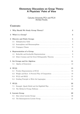
  • 23. The fundamental representation 3 is complex, i.e., inequivalent to ¯3. The states are labeled by the weights, the eigenvalues corresponding to X3 and X8. Note that λ1, λ2, and λ3 constitute an SU(2) in the 1-2 block. 7.1 Example: Quark Model and the Eightfold Way For concreteness, let us denote the three states of 3 by u, d, and s respectively, with or- thonormal eigenvectors: u =    1 0 0    , d =    0 1 0    , s =    0 0 1    . (86) These states are labeled by the third component of isospin, which is nothing but the entries of X3, and a quantum number called strangeness, which is a scaled variant of X8. Strong hypercharge is defined as 2X8/ √ 3, and subtracting baryon number (1/3 for all quarks) we get what is known as the strangeness: S = 2 √ 3 X8 − 1 3 . (87) Thus, for the three quarks, the I3-S assignments are as follows: u = 1 2 , 0 , d = − 1 2 , 0 , s = (0, −1) . (88) The weight diagram is shown in fig. 1. For the antiquarks, which live in ¯3, the assignments are just opposite. What happens when we combine 3 and ¯3? From a physics point of view, that is a combination of a quark and an antiquark, and should give some mesons. The question is: how do these mesons transform under SU(3)? S T3xx x 1/2,0−1/2,0 0,−1 ud s S T3 −1/2,0 1/2,0 u d sx 0,1 xx _ _ _ Figure 1: 3 and ¯3 of SU(3). Note that due to a scaling of X8 to S, the centre of mass of the two triangles are not the same. This would have been the case if we drew the triangles in X3-X8 plane. We follow the same principle of composition: take the antiquark triangle and place its centre of mass on the three vertices of the quark triangle. The resulting regular hexagon is shown in fig. 2. There are six states at the corners of the hexagon, and three in the middle. The names of the mesons are the standard ones used by particle physicists. There are a few points to note. 23
  • 24. ππηπ KK KK + − 0 η + − 0 0 ____ T S 310−1 1 −1 Figure 2: Composition of 3 and ¯3 of SU(3). • If we worked with only u and d quarks, that would have been an SU(2) doublet of isospin, and so among the composites, I should have a triplet. Experimentally, the middle member of the triplet happens to be π0 , see eq. (79) for the explicit wavefunc- tions. An SU(2) isospin transformation can be performed by the interchange of u and d, i.e., a shift along the horizontal line (that is obvious, S cannot change, since both quarks have zero strangeness). A look at fig. 2 immediately tells you that there are two more SU(2) doublets: K0 and K+ , and their antiparticles, K0 and K− . • The roots of SU(3) take one weight to the other. So they should act along the sides of the hexagon, and all members at the sides must belong to the same multiplet. By the isospin argument, π0 should also belong to the same multiplet. So what are the irreducible representations: 7 ⊕ 2, or 7 ⊕ 1 ⊕ 1, or what? The answer is that for any SU(n), n ⊗ ¯n = n2 − 1 ⊕ 1. (How do we know this, at least for SU(3)? We will see soon how to have an algorithm for getting the irreducible representations.) So the decomposition is 8⊕1. The singlet is one which does not transform under SU(3), and hence must be symmetric in the three quarks and antiquarks. This state is labeled as η′ = 1√ 3 u¯u + d ¯d + s¯s . From the T3 and S quantum numbers, it is one of the states at the middle of the hexagon. The third state must be an orthogonal one to this and π0 , and can be obtained by the standard Gram-Schmidt method: η = 1√ 6 u¯u + d ¯d − 2s¯s 6 . • These nine lowest mass meson states can be divided into an octet and a singlet. There are three different sets of raising and lowering operators for the octet (they have no effect on the singlet state). One of them is the set of isospin raising or lowering operators, obtained from a combination of X1 and X2. The other two sets are called U-spin and V-spin respectively. V-spin operators are those obtained from X4 and X5, 6 I have cheated you a bit. The actual singlet and octet states are not the physical states η′ and η; rather, the latter are a combination of the former states. However, the mixing angle is small, so for the group theory purpose, if not for particle physics purpose, the assignment that I use will do. 24
  • 25. and can change an up quark to a strange quark and vice-versa. U-spin operators, obtained from X6 and X7, take a d quark to an s quark and back. Note that only U-spin does not change the charge of the quarks and hence of the mesons. 7.2 The Method of Young Tableaux This is the most elegant method to get the irreducible representations out of a composite. The mathematical background is somewhat complicated, and needs tensor algebra, so we will skip that here. This forces us to state only the basic rules of the game. The algorithm goes like this: 3 3 8 1 6 10 __ Figure 3: Some simplest SU(3) representations. Figure 4: A ‘big’ tableau, with p = 2 and q = 1. • Each representation of SU(3) (well, there is nothing special about SU(3), it can be generalised for any SU group) is pictured as a set of boxes, as shown in fig. 3 and fig. 4. This does not mean that a box corresponds to a wave function. Rather, the whole set, and its symmetry and antisymmetry properties, are depicted by the box pattern. The boxes must be – left-aligned; – arranged in such a way that the number of boxes does not increase as one goes down the columns (it may decrease or remain constant); – arranged in not more than three rows (this number depends on what SU group you choose; e.g., it will be five for SU(5)). 25
  • 26. • With such a pattern, let the difference between the number of boxes in the first and the second rows be p, and the difference between the second and the third rows be q. The dimensionality of the representation, denoted also as (p, q), is given by d = 1 2 [(p + 1)(q + 1)(p + q + 2)] . (89) Thus, a single box corresponds to (p, q) = (1, 0), and hence it has dimensionality 3; this is the fundamental representation of SU(3). The arrangement of two boxes in a column is (p, q) = (0, 1) and hence this is ¯3. The representations with p = q are the real representations; setting aside p = q = 0, which is the singlet of dimensionality 1, the lowest possible arrangement is (p, q) = (1, 1) ⇒ 8, the adjoint representation. (What is the dimensionality of the representation shhown in fig. 4?) • Three boxes in a column has p = q = 0. This is a singlet, and anything multiplied by unity is the same thing, so composition with a singlet is trivial. That is why this particular combination is, so to say, irrelevant; to get the dimensionality of a representation, we can add or subtract at our will as many number of three boxes in a column as we wish. In any combination, if you happen to have any such arrangement, you can easily scratch that off (unless you require them to have a feeling of what q will be). • Boxes in a row denote a symmetric combination of wavefunctions, and boxes in a column denote antisymmetric combination. While trying a composition, one must remember that symmetrised wavefunctions cannot be antisymmetrised, and vice versa. Boxes which are not in a particular row or column can be placed anywhere. A singlet is a state where the whole wavefunction is antisymmetric, i.e., it picks up a minus sign every time you interchange two states: |1 = 1 √ 6 (uds − dus + dsu − sdu + sud − usd) . (90) This is a linear combinaion of six wavefunctions; the first means that u is at position 1, d at 2, and s at 3. Interchange u and d and the whole wavefunction picks up a minus sign. The prefactor is for normalisation. • Double counting must be avoided. aX b == + + + a b a b a b b a 3 3 __ 1 8 Figure 5: An instructive but unsmart way to get 3 ⊗ ¯3. 26
  • 27. == +X 3 _ 3 8 1 Figure 6: The same composition can be obtained in a smarter way. Fortunately, the most important applications of SU(3) Young tableaux are the most simple ones. As an example, let us try to emulate Murray Gell-Mann in his search for the eightfold way. Fig. 5 shows the final result, but we have to go through the intermediate steps. • Unless this is a very simple composition (like joining two 3s), always label all the boxes of the second (i.e., the one on the right hand side) tableau. Label all boxes of a row in an identical way, but different from boxes in another row. For example, label all boxes of the first row by a, and all in the second row by b (the third row never counts; a full column can always be eliminated). • Take one box from the first row and join it in as many possible ways with the first tableau as possible. Of course, you have to join it only on the right hand side or below. Remember that the number of boxes in each row of this combined representation (even if this is an intermediate step) should never increase as you go down the columns. The operation gives nothing but 3 ⊗ 3 = 6 ⊕ ¯3. This intermediate step, however, is not shown in fig. 5. • Repeat this step until you finish of all the boxes in the first row. Then start the game with the boxes in the second row. Here you must be a little careful. Naively, you would have obtained all the four combinations shown in fig. 5. But two of them are not allowed: boxes a and b are in a column, i.e., in an antisymmetric combination, and cannot be symmetrised, i.e., put in a row. Also, in no tableaux one should have b sitting above a (they can be in the same row, if initially they belong to different columns and hence without any antisymmetry property). This is nothing but avoiding double counting. Thus, two of the boxes are ruled out, and we get the required decomposition. • However, a smarter way is shown in fig. 6; I can always take 3 as my second box. Then only two tableaux appear and there is no question of any double counting! • As a further example, let us consider the combination of three quarks: 3 ⊗ 3 ⊗ 3. This is shown in fig. 7. The process is a two-step one; first we combine two 3s, and then combine the result with the last 3. Mathematically, we write 3 ⊗ 3 ⊗ 3 = (6 ⊕ ¯3) ⊗ 3 = 10 ⊕ 8 ⊕ 8 ⊕ 1. (91) The 3 × 3 λ matrices satisfy the following relations: [λa, λb] = 2ifabcλc, {λa, λb} = 4 3 δab1 + 2dabcλc, Tr(λaλb) = 2δab. (92) 27
  • 28. X X == ( + ) X == + + + 3 3 3 6 3 _ 3 10 8 8 1 Figure 7: Combination of three 3s. In the quark model, this gives the baryons. The completeness relation is (λa)ij(λb)kl = − 2 3 δijδkl + 2δilδjk (93) where i, j, k, l = 1, 2, 3. The quadratic and cubic Casimir operators are defined as C2(R)1 ≡ 8 a=1 (Xa)2 (R), C3(R)1 ≡ 8 a,b,c=1 dabcXa(R)Xb(R)Xc(R), (94) where R is the dimension of the representation (3 for fundamental) and Xa = λa/2. It can be shown that C2(p, q) = 1 3 p2 + pq + q2 + 3p + 3q , C3(p, q) = 1 18 (p − q)(2p + q + 3)(2q + p + 3). (95) This gives, e.g., C2(3) = 4/3, C2(8) = 3. Now, some important relations. From eq. (93), we have (λa)ij(λa)jl = − 2 3 + 2 × 3 δil = 4C2(3)δil. (96) From the definition of the adjoint representation (Xa)bc = −ifabc, facdfbcd = C2(8)δab = 3δab. (97) Q. Perform the topnotch exercise: 8 ⊗ 8 = 27 + 10 + 10 + 8 + 8 + 1. Be careful to avoid double counting. Also preserve the symmetry and the antisymmetry properties. 28
  • 29. Q. Show that fabcλbλc = iC2(8)λa. (Hint: write λbλc = 1 2 [λb, λc] since fabc is completely antisymmetric, and then use eq. (97).) Q. Justify the steps: λbλaλb = 1 2 (λb[λa, λb] − [λa, λb]λb + λbλbλa + λaλbλb) = 4C2(3)λa + ifabc[λb, λc] = 4 C2(3) − 1 2 C2(8) λa. (98) 8 Lorentz Group Let us recall that the ordinary rotation groups SO(2) and SO(3) have one and three genera- tors respectively. They are the groups for two-dimensional and three-dimensional rotations. The generator of SO(2) is just σ2, while SO(3) has three generators J1, J2, and J3 satisfying [Ji, Jj] = iǫijkJk. Now let us consider the Lorentz transformations (LT). We take the metric to be Minkowski, with gµν = diag(+1, −1, −1, −1), and set c = 1. The three generators for rotation will be still there, but they are enlarged, e.g., J1 =      0 0 0 0 0 0 0 0 0 0 0 −i 0 0 i 0      , (99) and permutations generate J2 and J3. The extra row and column of zeroes remind us that the space-time is four-dimensional, (x0 , x1 , x2 , x3 ), and rotations do not affect the time dimension. The Jis satisfy the same SO(3) algebra as before. However, the group has three more generators, boosts along the three spatial axes, denoted by Ki. Consider a boost in the x ≡ x1 direction, which can be written as t′ = t cosh φ − x sinh φ, x′ = x cosh φ − t sinh φ , (100) where tanh φ = v. For small φ, this becomes t′ = t − xφ, x′ = x − tφ, so that the generator K1 has the form K1 =      0 −1 0 0 −1 0 0 0 0 0 0 0 0 0 0 0      . (101) (What should be the forms of K2 and K3?) Note that a finite transformation is given by exp(αaKa); there is no i, and the αs are real, so the group is a noncompact one. Thus, it need not be represented by unitary matrices. However, to work out the group algebra, we should express the group operations in an identical way: Λ(θa, αa) = exp(iθaJa + iαaKa) , (102) where Ka = iKa, and thus, for example, K1 =      0 i 0 0 i 0 0 0 0 0 0 0 0 0 0 0      . (103) 29
  • 30. Now compute by brute force to verify that [Ji, Jj] = iǫijkJk, [Ji, Kj] = iǫijkKk, but [Ki, Kj] = −iǫijkJk. (104) This last commutator is interesting: the commutator of two boosts is a rotation. In other words, if you boost some object along the x-axis, and then along the y-axis, but boost it back to the original position by first applying a reverse boost along the y-axis and then along the x-axis, you will find that the body has undergone a rotation about the z-axis! This is known as the Thomas precession. The Lorentz group, denoted by SO(3, 1), is reducible 7 . This is one of its most important features. Construct the generators J±i = 1 2 (Ji ± iKi). Check that [J+i, J+j] = iǫijkJ+k, [J−i, J−j] = iǫijkJ−k, and [J+i, J−j] = 0. (105) The algebra falls apart in two SU(2)s. To be very precise, SO(3, 1) is isomorphic to SU(2) ⊗ SU(2). Therefore, any representation of the Lorentz group can be written as (j1, j2), a pair of SU(2) representations, with a dimensionality of (2j1 +1)(2j2 +1). With in- creasing dimensionality, the representations are (0, 0), (1/2, 0) and (0, 1/2), (1, 0) and (0, 1), (1/2, 1/2), and so on. The Lorentz scalar is (0, 0), and the fundamental representation is the 4-dimensional Lorentz vector (1/2, 1/2). Why, then, we use a four-component Dirac spinor, instead of a two-component Weyl spinor? The reason is parity: under parity operation, Ji does not change sign (angular momentum is an axial vector) but Ki does, and so J±i → J∓i. In other words, (1/2, 0) ↔ (0, 1/2). These are known as the left-chiral and the right-chiral representations respectively. But electrodynamics is invariant under parity, so we must have some wavefunction that is a combination of two SU(2) doublets. If we have some theory that violates parity, we can do with two-component spinors, and indeed under weak interaction, the two Weyl doublets behave differently. 8.1 More about Lorentz Groups There is another way to look at the Lorentz groups. What we have just discussed is in fact only a restricted subset of the full group. A homogeneous Lorentz group is characterised by the coordinate transformation x′µ = Λµ ν xν (106) or, in matrix notation, x′ = Λx. This must leave the quadratic form x2 = xµ xµ = (x0 )2 −(xi )2 invariant. All entries in the matrix Λ are real, so the condition of invariance of the quadratic form can be written as Λµ ν Λν ρ = δµ ρ . (107) This can be written as Λµ ν gµσΛσ ρ = gνρ, (108) or, in other words, since Λµ ν = (ΛT )ν µ, ΛT gΛ = g, (109) 7 Technically, what we are interested in is a subset of the full Lorentz group that is continuously connected to the identity. Sometimes called the restricted Lorentz group, this is denoted by SO+ (3, 1), but we will not be that fussy about mathematical notations. 30
  • 31. where the superscript T denotes the transposed matrix. It follows from this equation that detΛ = ±1 and hence every homogeneous LT has an inverse transformation. The product of two LTs is another LT, and hence LTs form a group. Obviously, the Lorentz group has a proper subgroup: the group of 3-dimensional rotation, SO(3). Setting ν = ρ = 0 in eq. (108), we get (Λ0 0)2 = 1 + 3 i=1 (Λi 0)2 ≥ 1, (110) so that Λ0 0 ≥ 1 or Λ0 0 ≤ −1. The first set is known as orthochronous LT, the second is non- orthochronous. Orthochronous LTs transform a positive time-like vector into another posi- tive time-like vector, and the set of all orthochronous LTs form a group: the orthochronous Lorentz group. (Why the non-orthochronous set is not a group?) Again, for both the choices of Λ0 0, detΛ can be +1 or −1. The subset with Λ0 0 ≥ 1 and detΛ = +1 is the group of restricted homogeneous LTs (this is the group we were discussing in the last subsection). All elements are continuously connected to identity. The other three subsets are obtained by adjoining the following transformations to the restricted homogeneous LT group: Space inversion (x0 → x0 , x → −x) : Λ(is) =      1 0 0 0 0 −1 0 0 0 0 −1 0 0 0 0 −1      , Time inversion (x0 → −x0 , x → x) : Λ(it) =      −1 0 0 0 0 1 0 0 0 0 1 0 0 0 0 1      , Space − time inversion (x0 → −x0 , x → −x) : Λ(ist) =      −1 0 0 0 0 −1 0 0 0 0 −1 0 0 0 0 −1      .(111) These subsets are disjoint and are not continuously connected to identity. Q. Convince yourself of the validity of eq. (108). Q. Which of the three improper LTs is orthochronous? 8.2 The Inhomogeneous Lorentz Group The inhomogeneous Lorentz group (also called the Poincar´e group) is characterised by the transformation x′µ = Λµ ν xν + aµ , (112) where aµ is a real four-vector. So this is nothing but a product transformation of a homo- geneous LT and a translation. Therefore it has ten generators, six from the homogeneous Lorentz group and four from translation, which are nothing but pµ . The algebra is enlarged by the commutators [pµ, pν] = 0, [Mµν, pσ] = i(gνσpµ − gµσpν), (113) where Mµν is the hermitian generators for homogeneous LT in xµ -xν plane. 31
  • 32. 9 Epilogue This is only a sketchy note. I have avoided detailed deductions as far as possible. You should not avoid them. You should definitely work out the problems, and think whenever you are expected to think. Remember that exploration of symmetries is what physics is mostly about. Group theory is a tool to help you, but it is not the physics itself. For those who wish to be condensed matter physicists, the discussion on discrete groups is terribly limited here. You will have to learn much more about the crystallographic point groups, but this note may act as a good starter. Be careful about the notation: I have used my own notations, which may not always tally with the standard ones. Fortunately, physics does not depend on notations, but communication skill may. The discussion on Lie groups is also far from exhaustive. There are a number of topics I have not touched, but you can always come back and read a good text if you need them. This discussion should be able to get you started in your course on nuclear or particle physics. Feel free to contact me if you wish. My office is always open for you, and so is my e-mail id: akphy@caluniv.ac.in . 32