Downloaded 57 times

![Sampling
44
© 1992-2008 R .C. Gonzalez & R.E. Woods
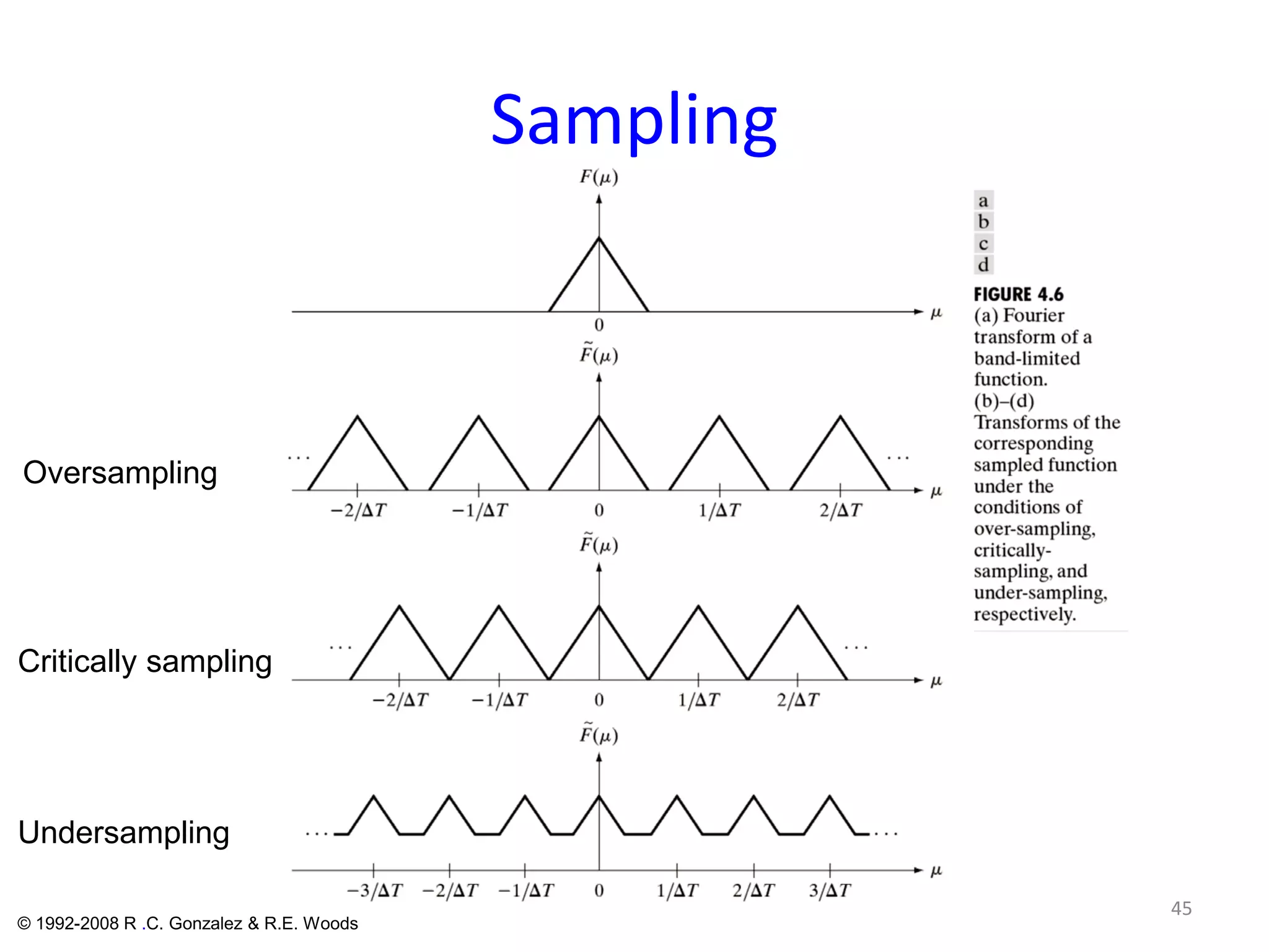
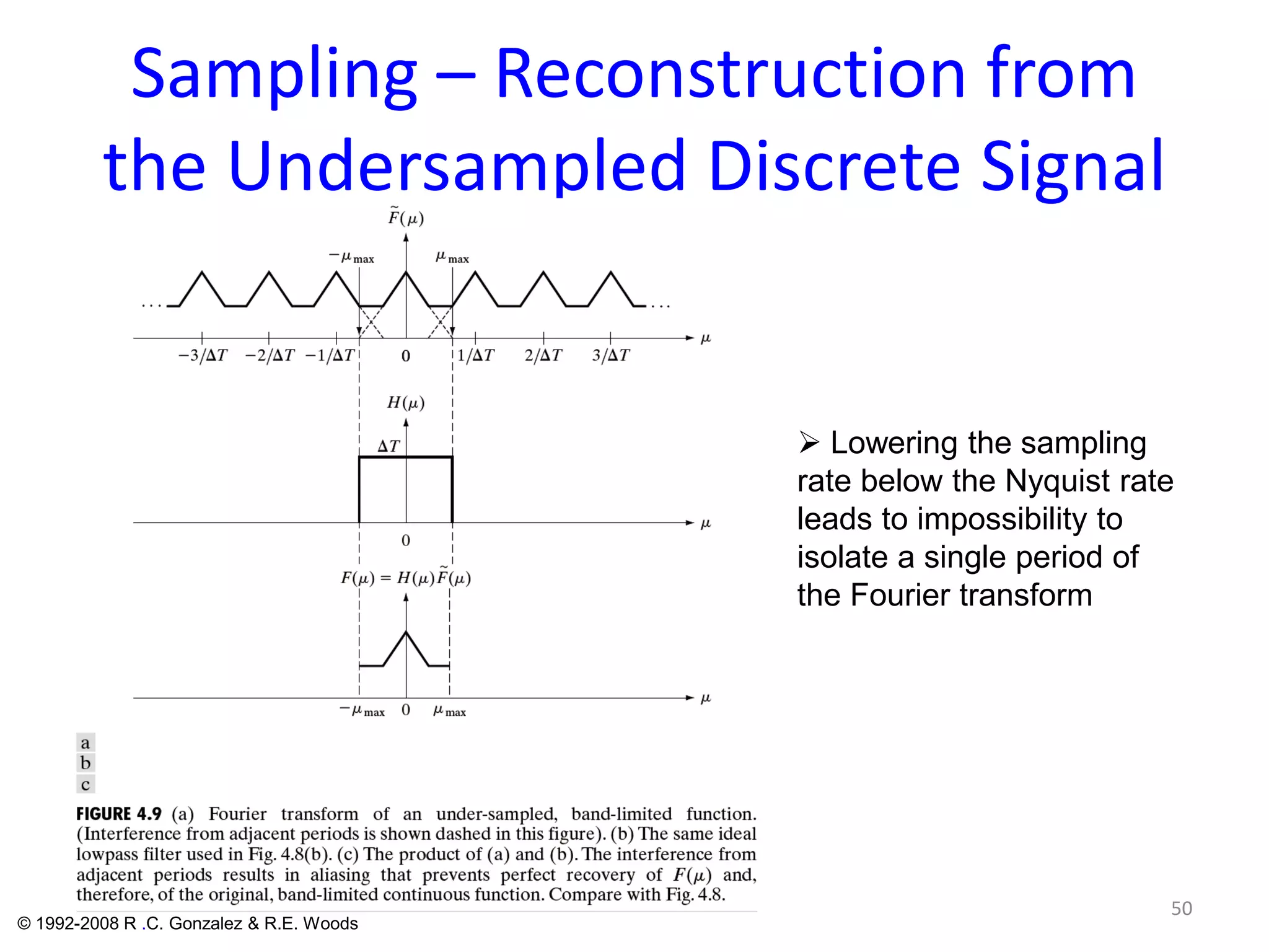
[ ]max max,µ µ− - The frequency range of
a band-limited signal
max
1
2
t
µ=
∆
- The Nyquist rate
To recover a signal from its
sampled representation, the
sampling rate must exceed the
Nyquist rate:
max
1
2
t
µ>
∆](https://image.slidesharecdn.com/yooex3fsacasyhtwx0jl-signature-0a8186d369408624cdd09d1ec93772439659798bf77cdb35dc7b4c2c066e57ab-poli-160109133314/75/Lecture-9-44-2048.jpg)

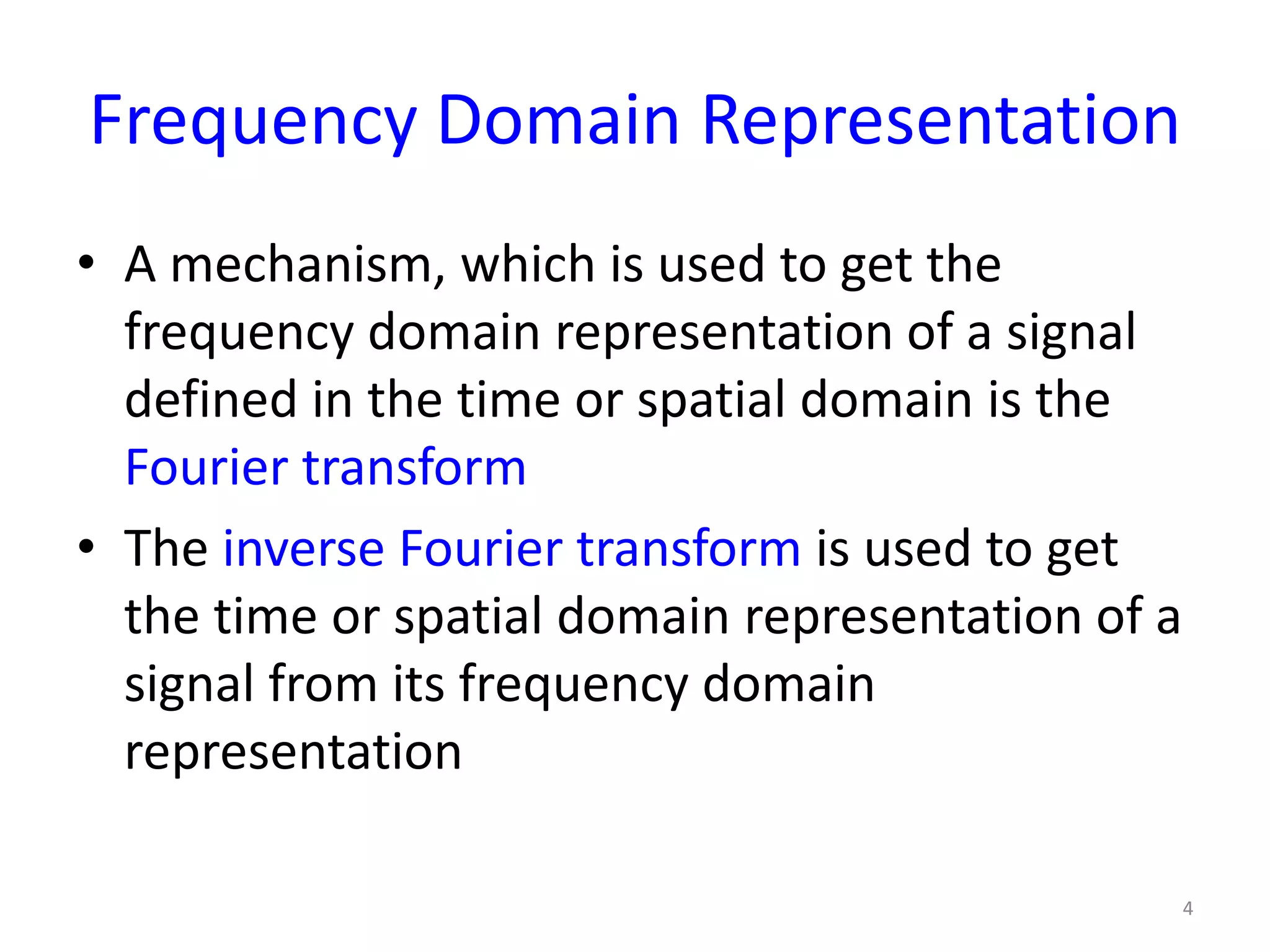
The document discusses frequency domain processing and the Fourier transform. It defines key concepts such as: - The frequency domain represents how much of a signal lies within different frequency bands, while the time domain shows how a signal changes over time. - The Fourier transform provides the frequency domain representation of a signal and is used to analyze signals with respect to frequency. Its inverse transform reconstructs the original signal. - The Fourier transform decomposes a signal into orthogonal sine and cosine waves of different frequencies, showing the contribution of each frequency component. This representation is important for signal processing tasks like filtering.
Introduces frequency domain processing and Fourier Transform for analyzing signals.
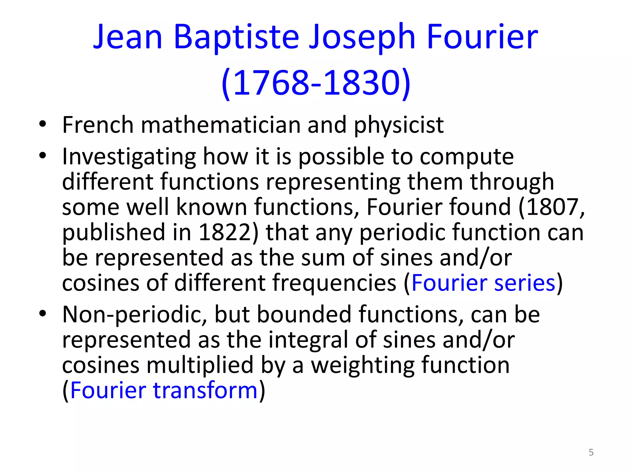
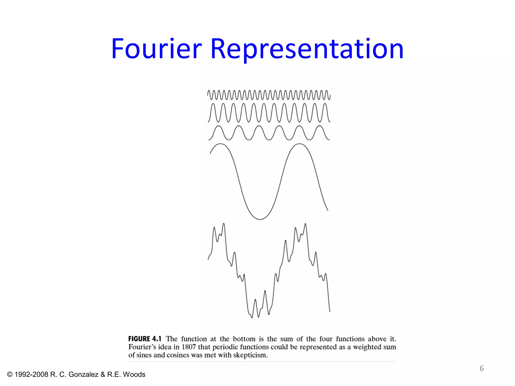
Discusses Jean Baptiste Joseph Fourier's contributions, periodic functions, and orthogonal functions in signal representation.
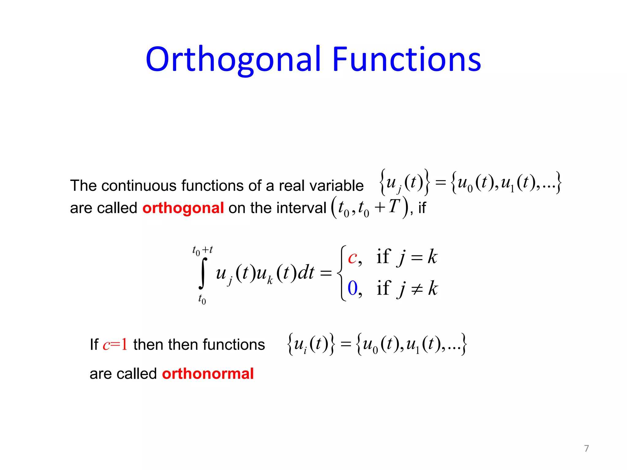
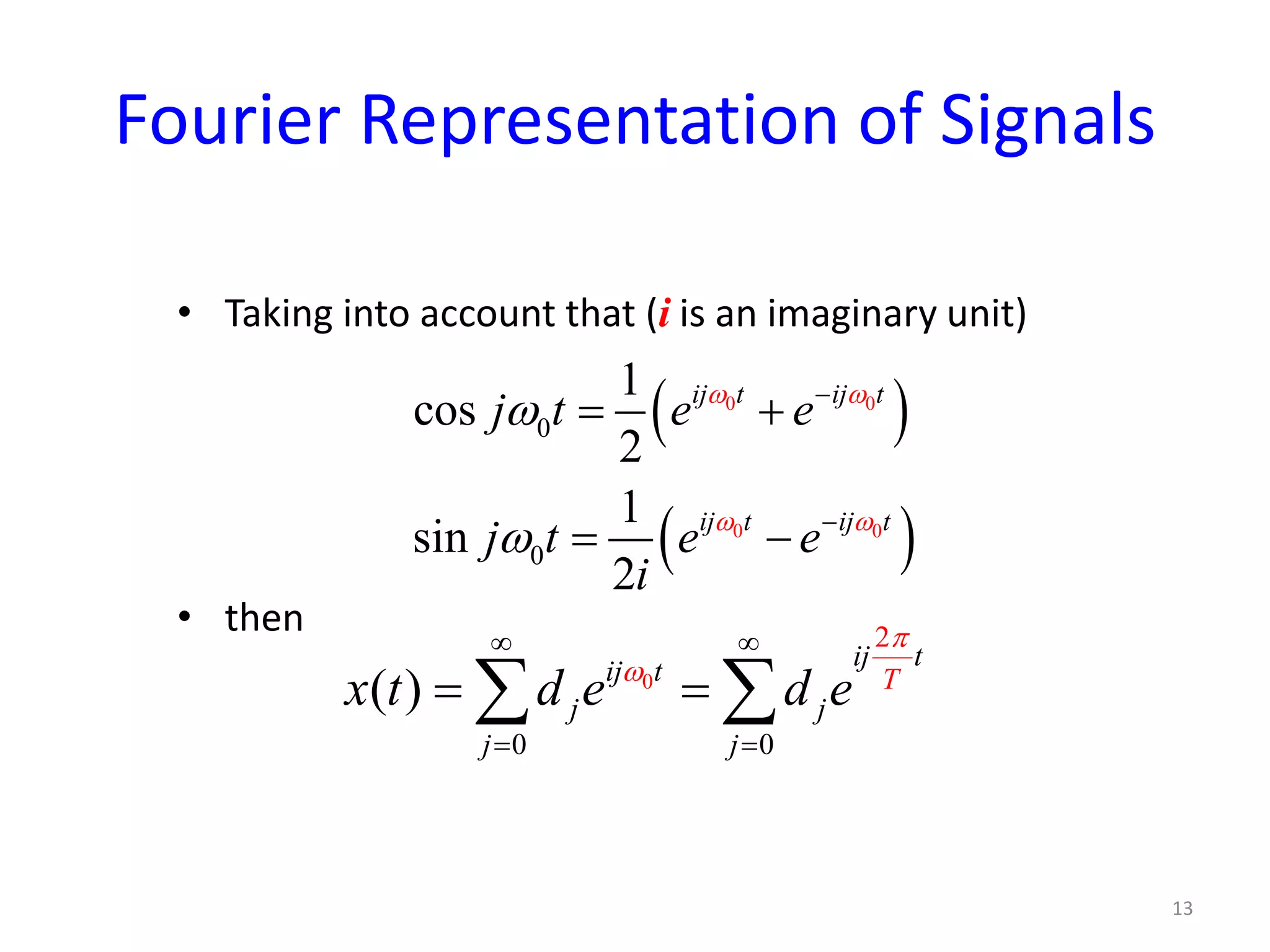
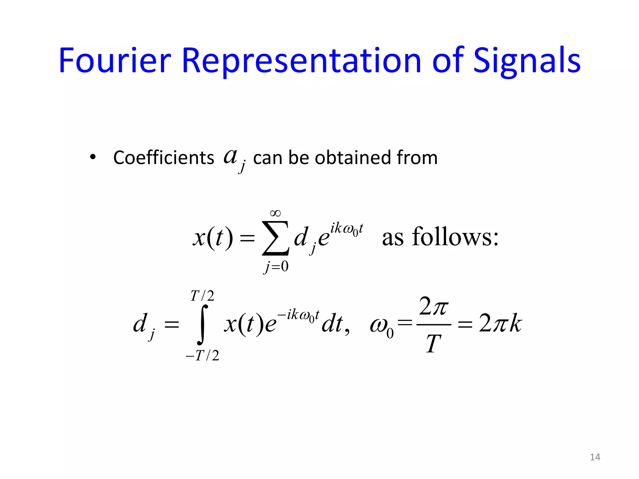
Explains how to represent signals using Fourier series in terms of orthogonal functions and coefficients.
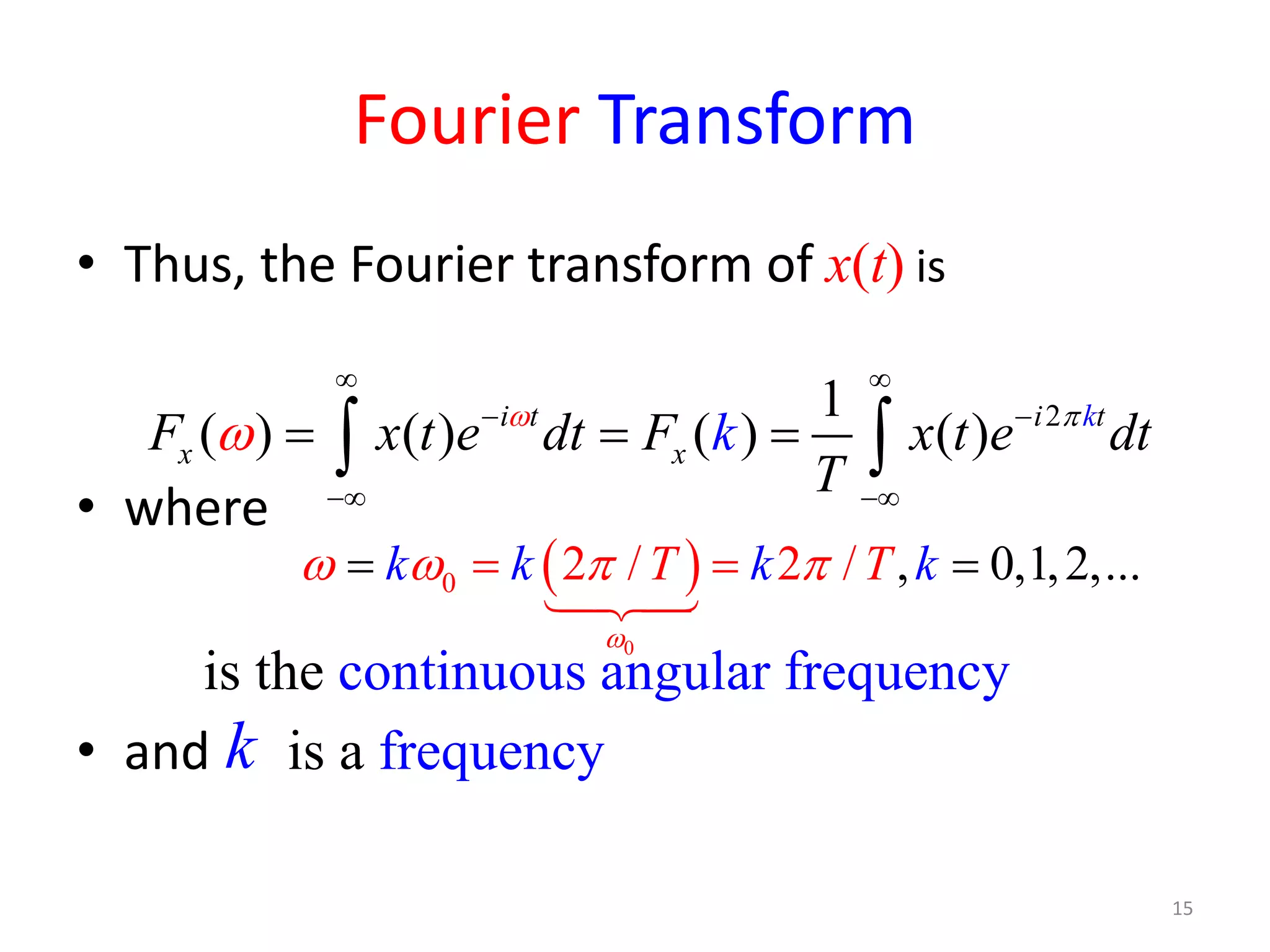
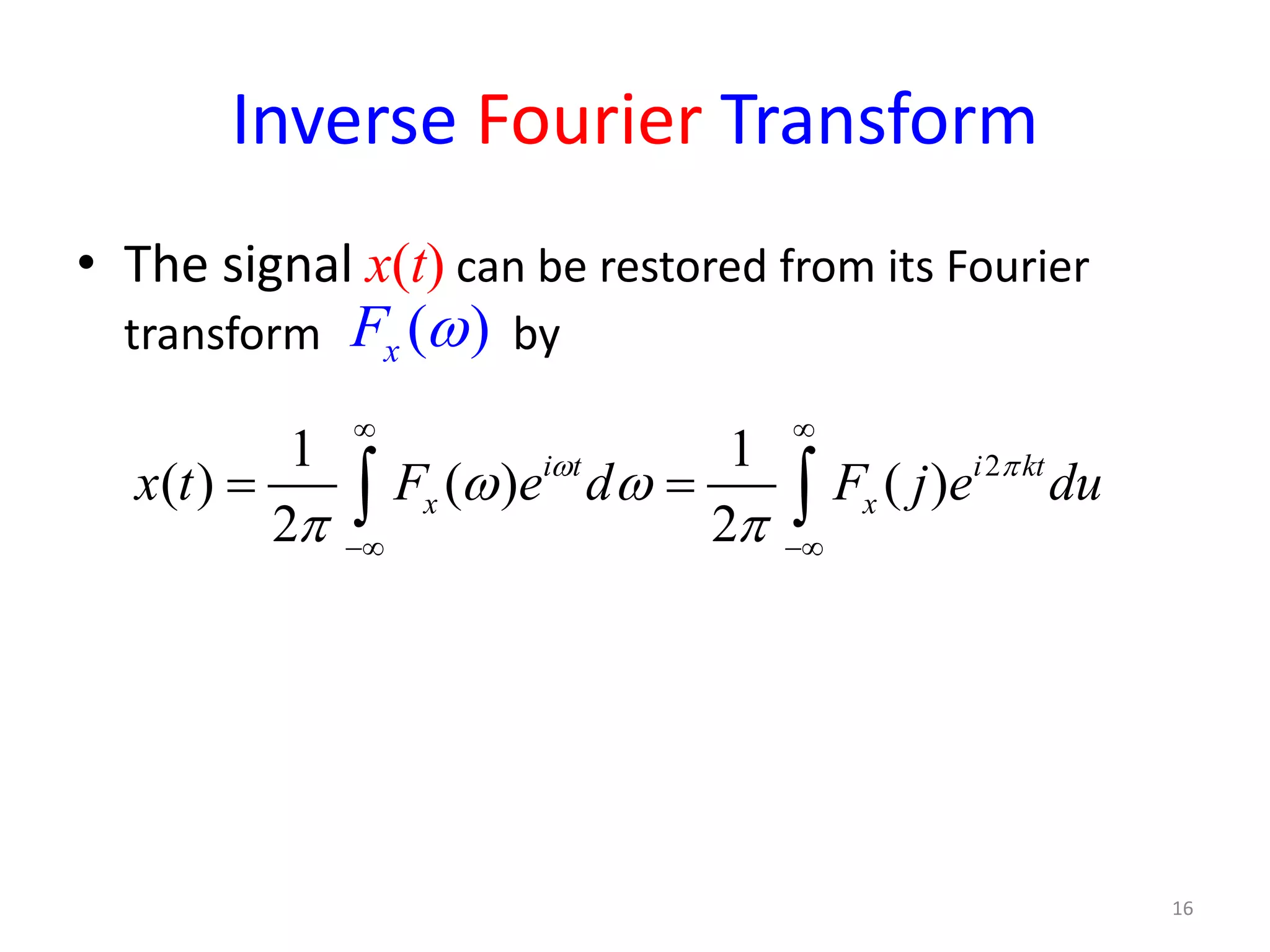
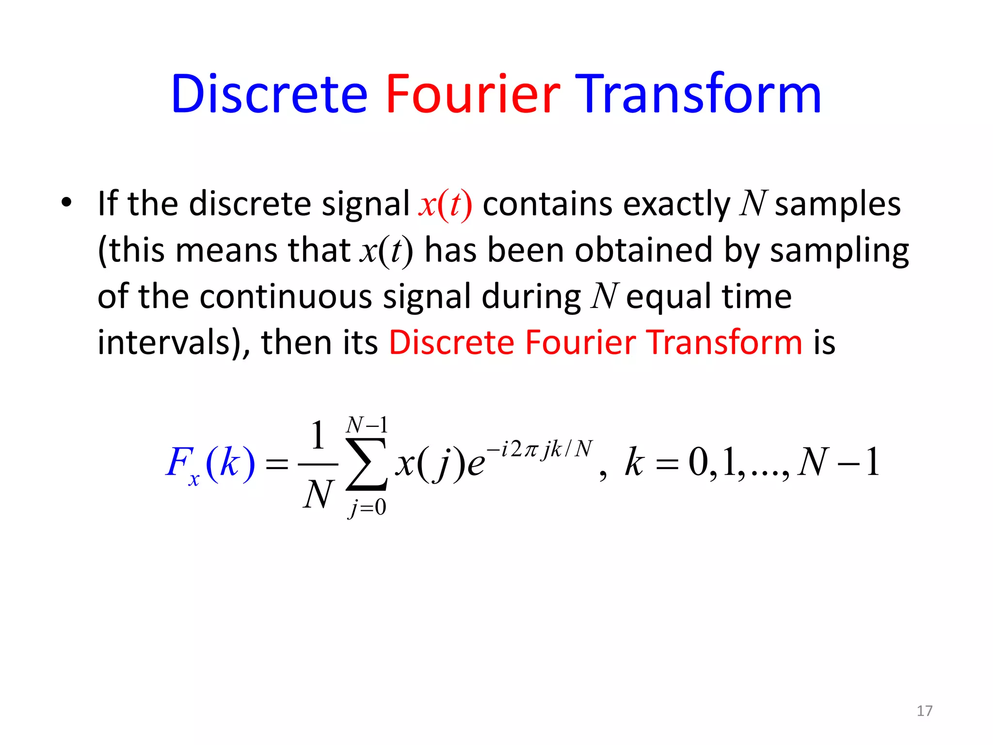
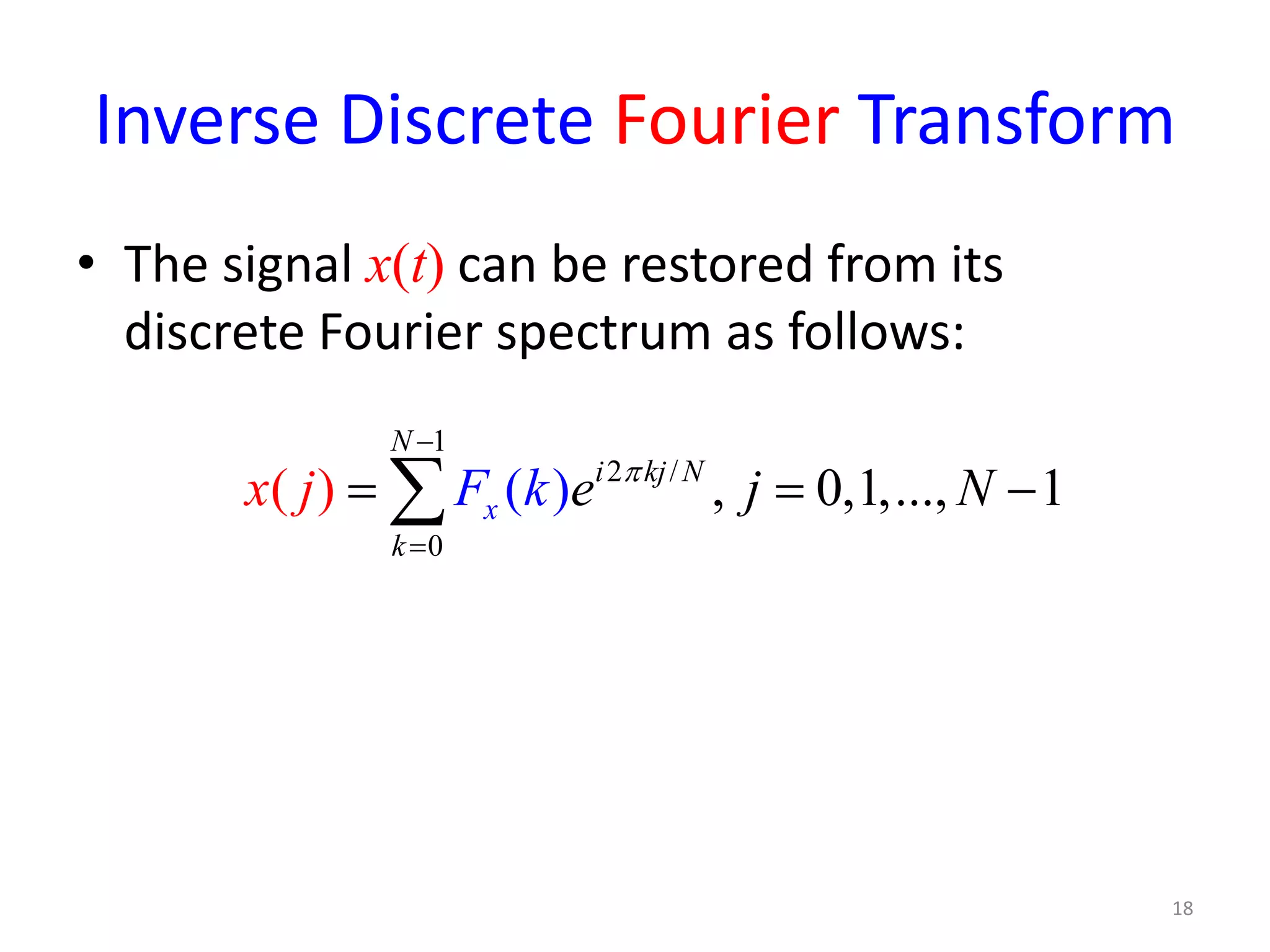
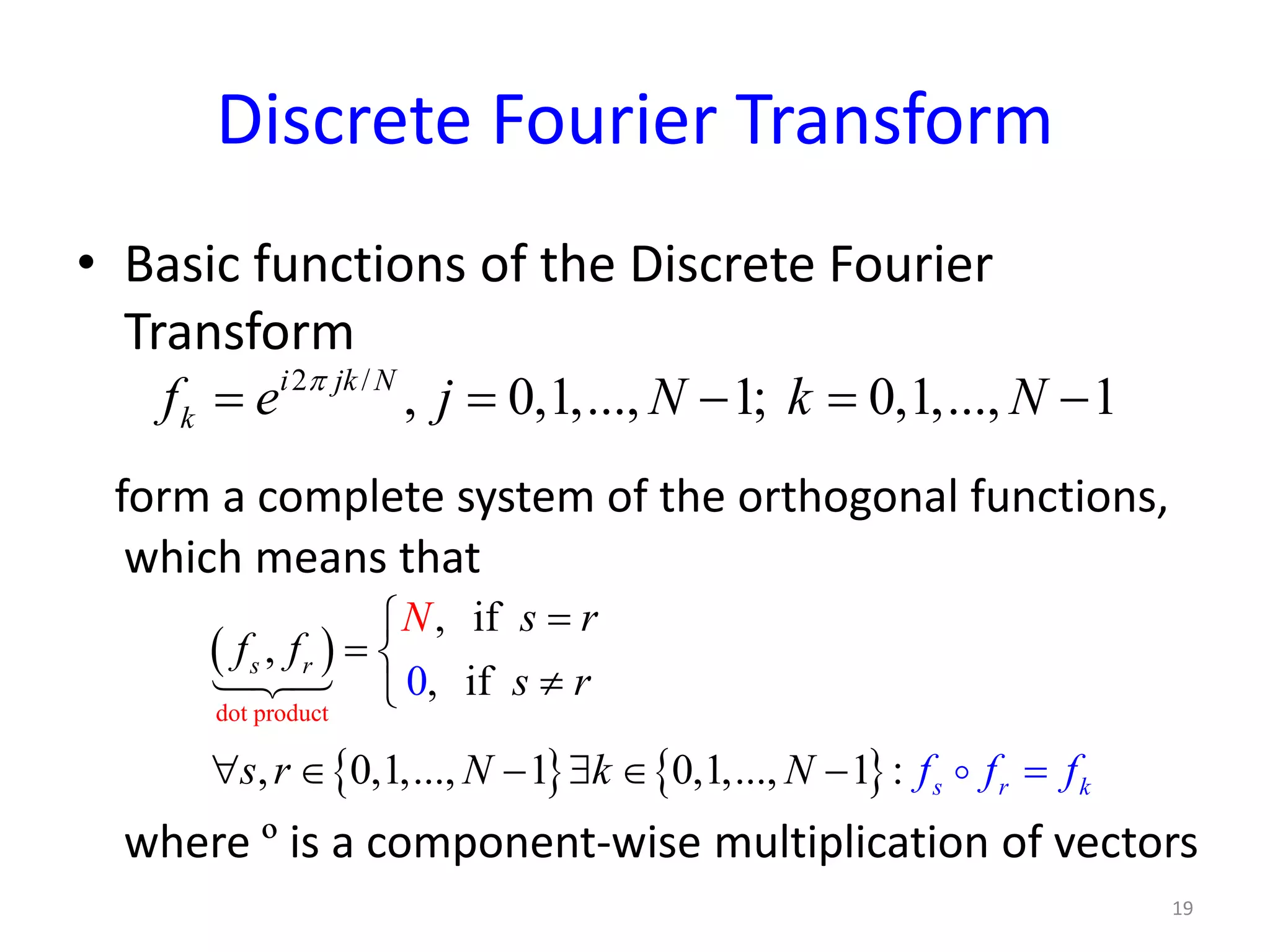
Defines Fourier Transform, Inverse Fourier Transform, and Discrete Fourier Transform to analyze signals.
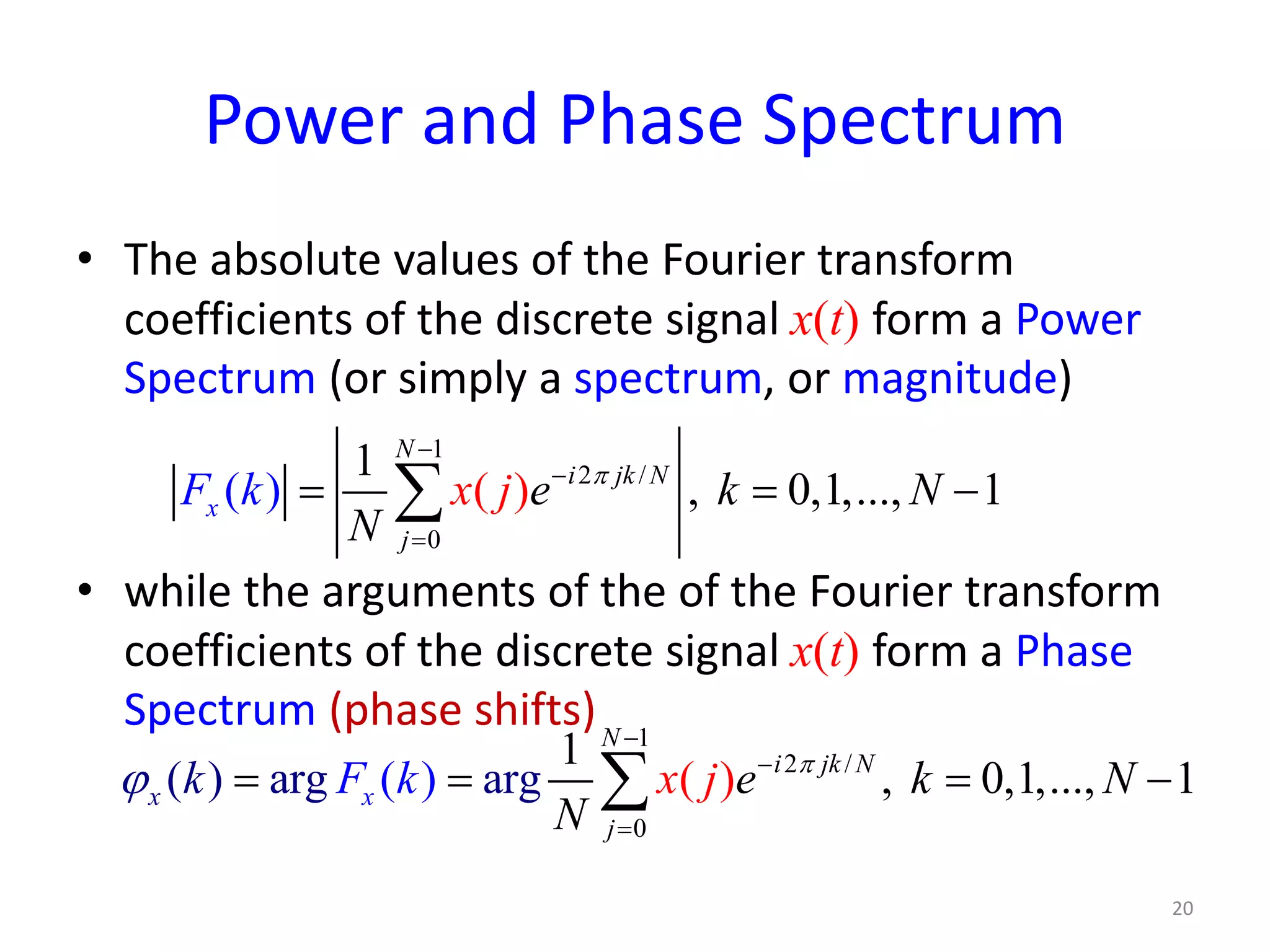
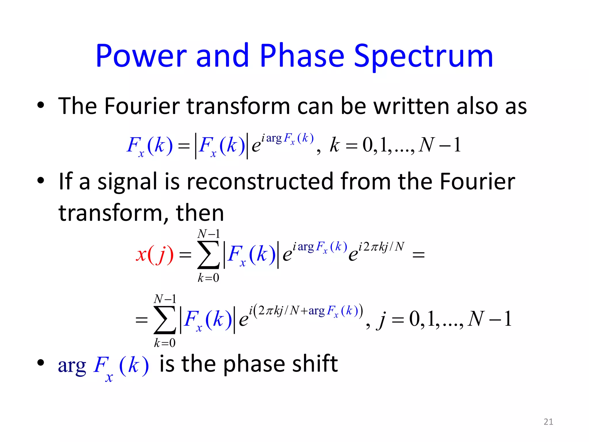
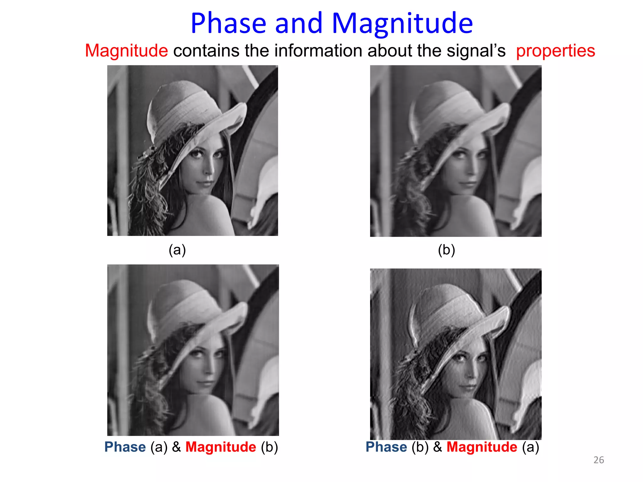
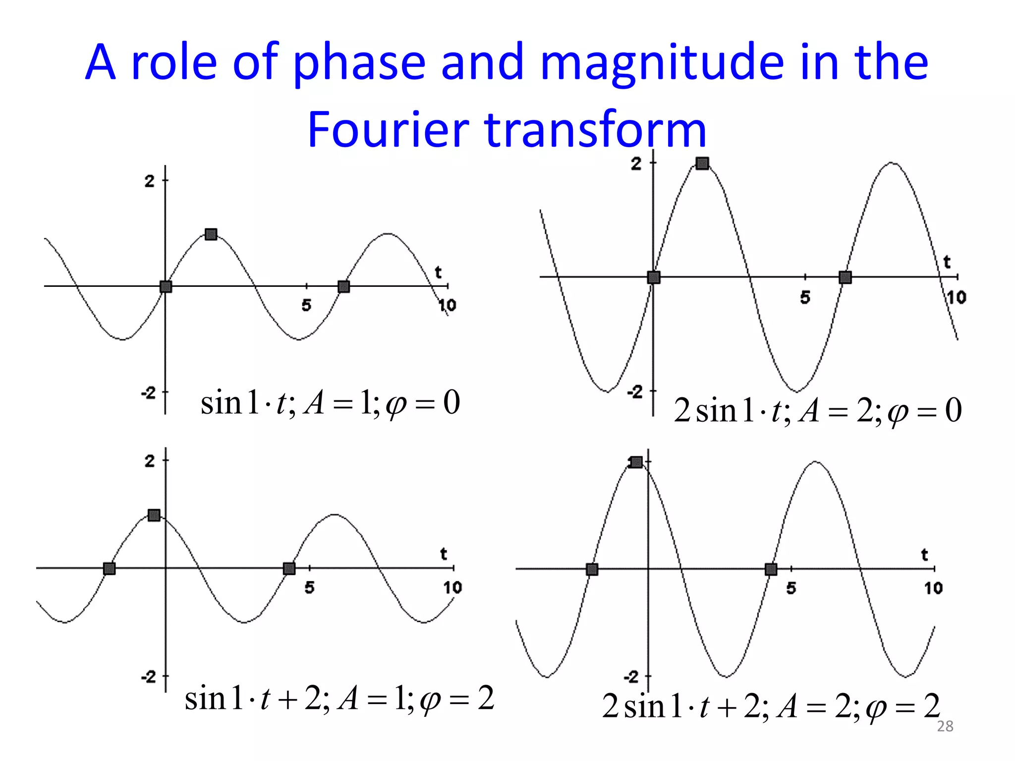
Discusses Power Spectrum and Phase Spectrum in analyzing signal properties and importance for image recognition.
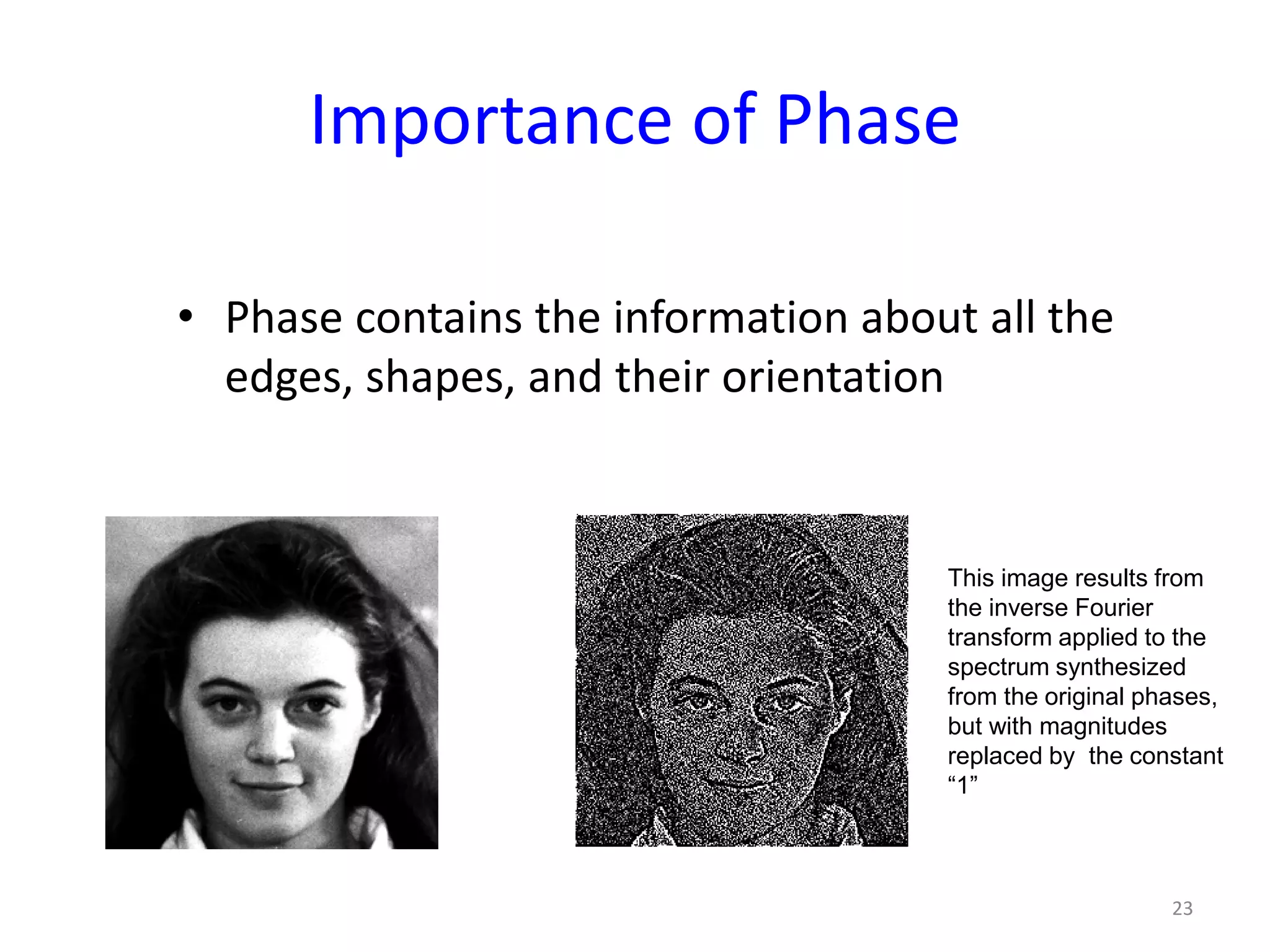
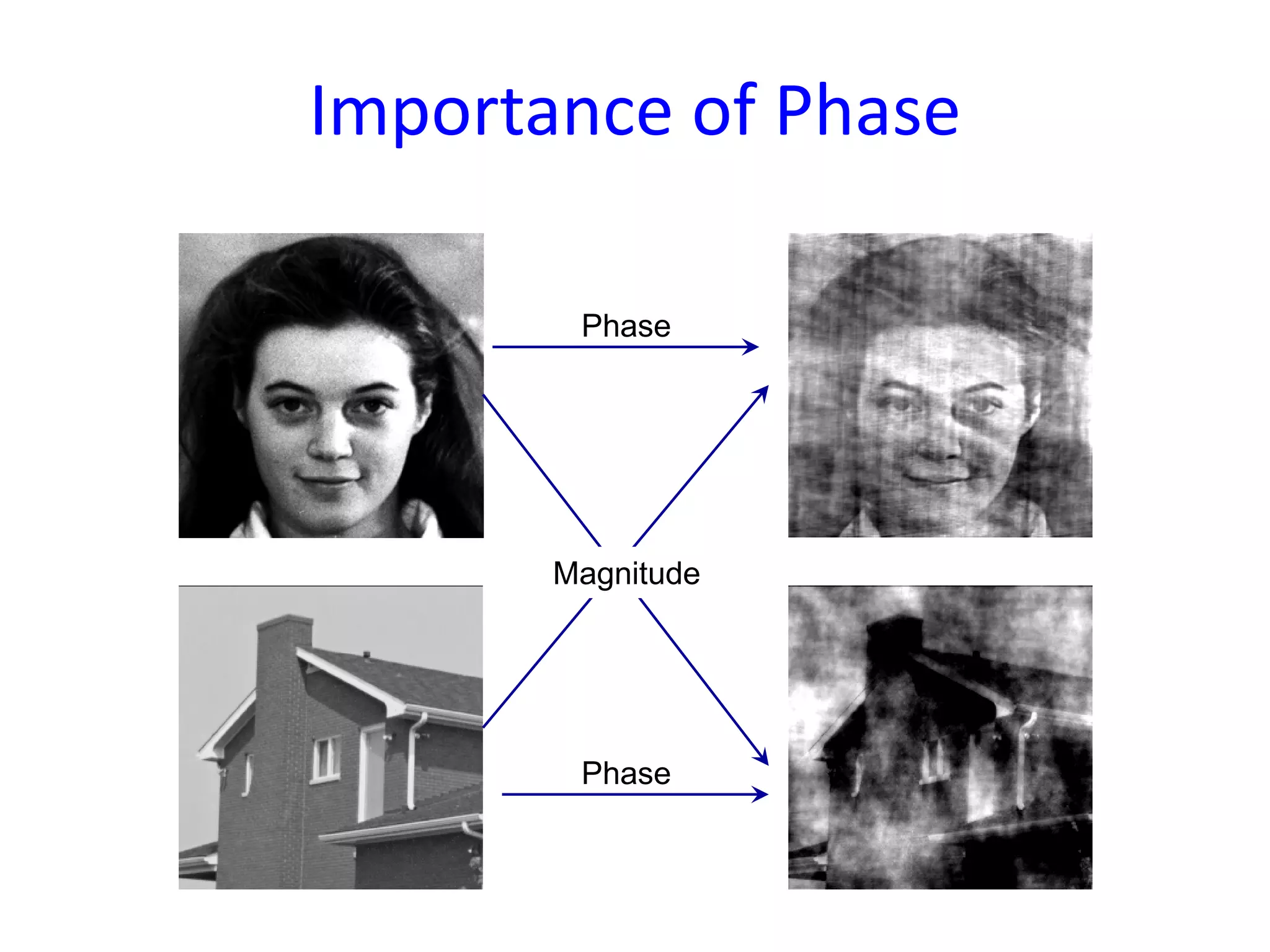
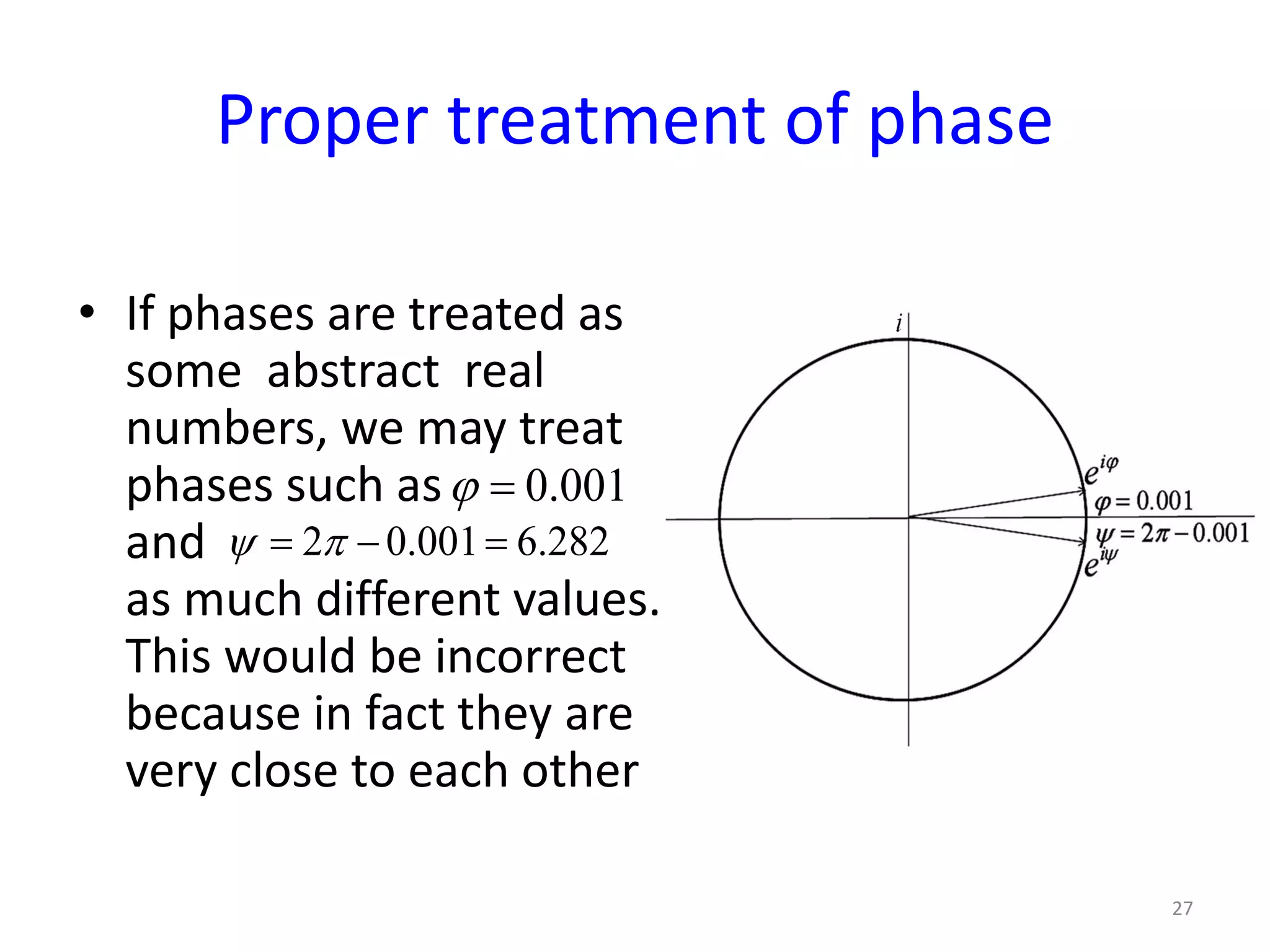
Highlights the significance of phase information over magnitude in reconstructing images and signal features.
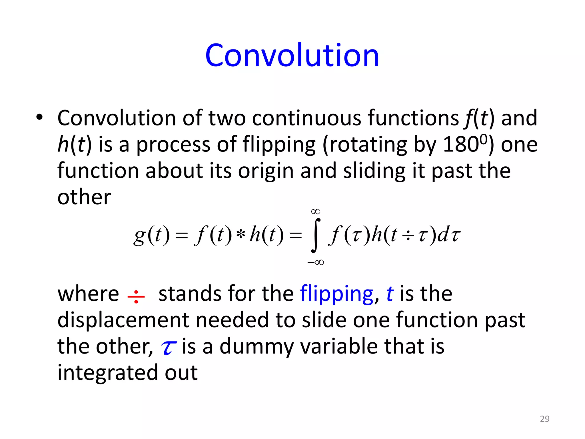
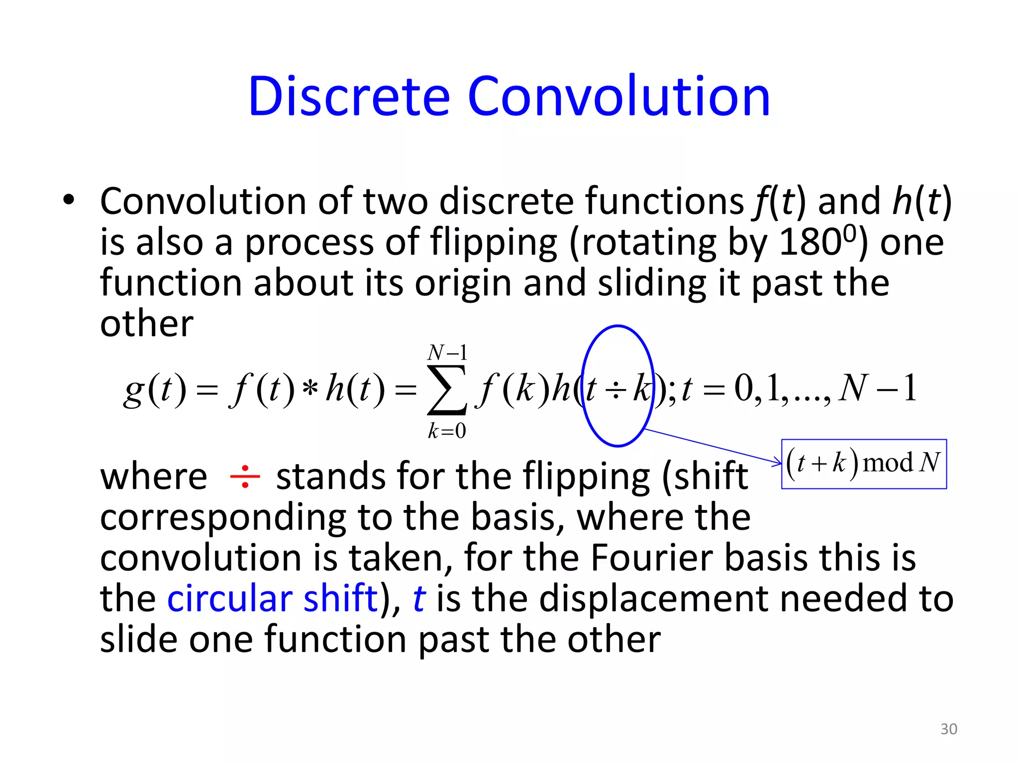
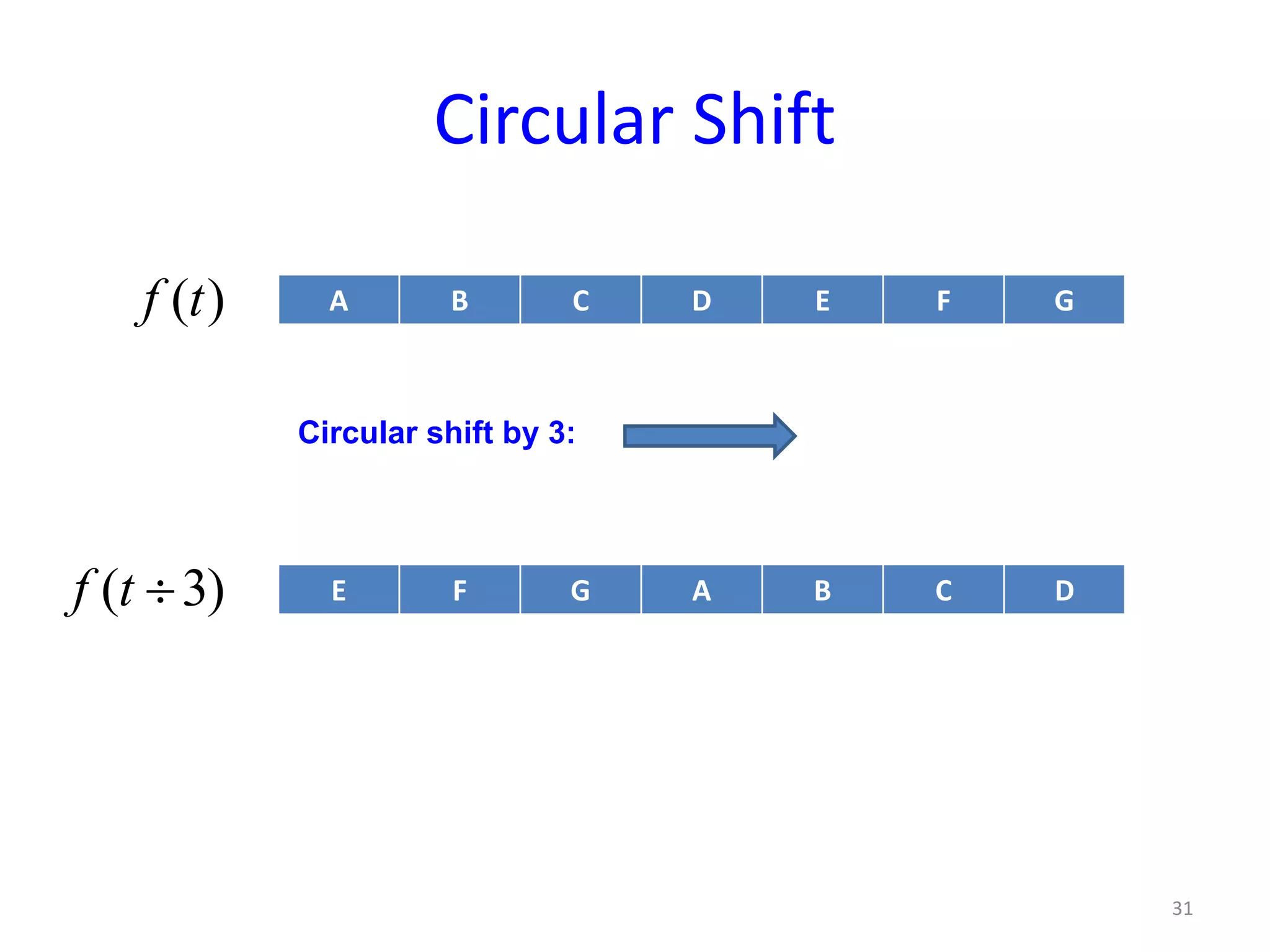
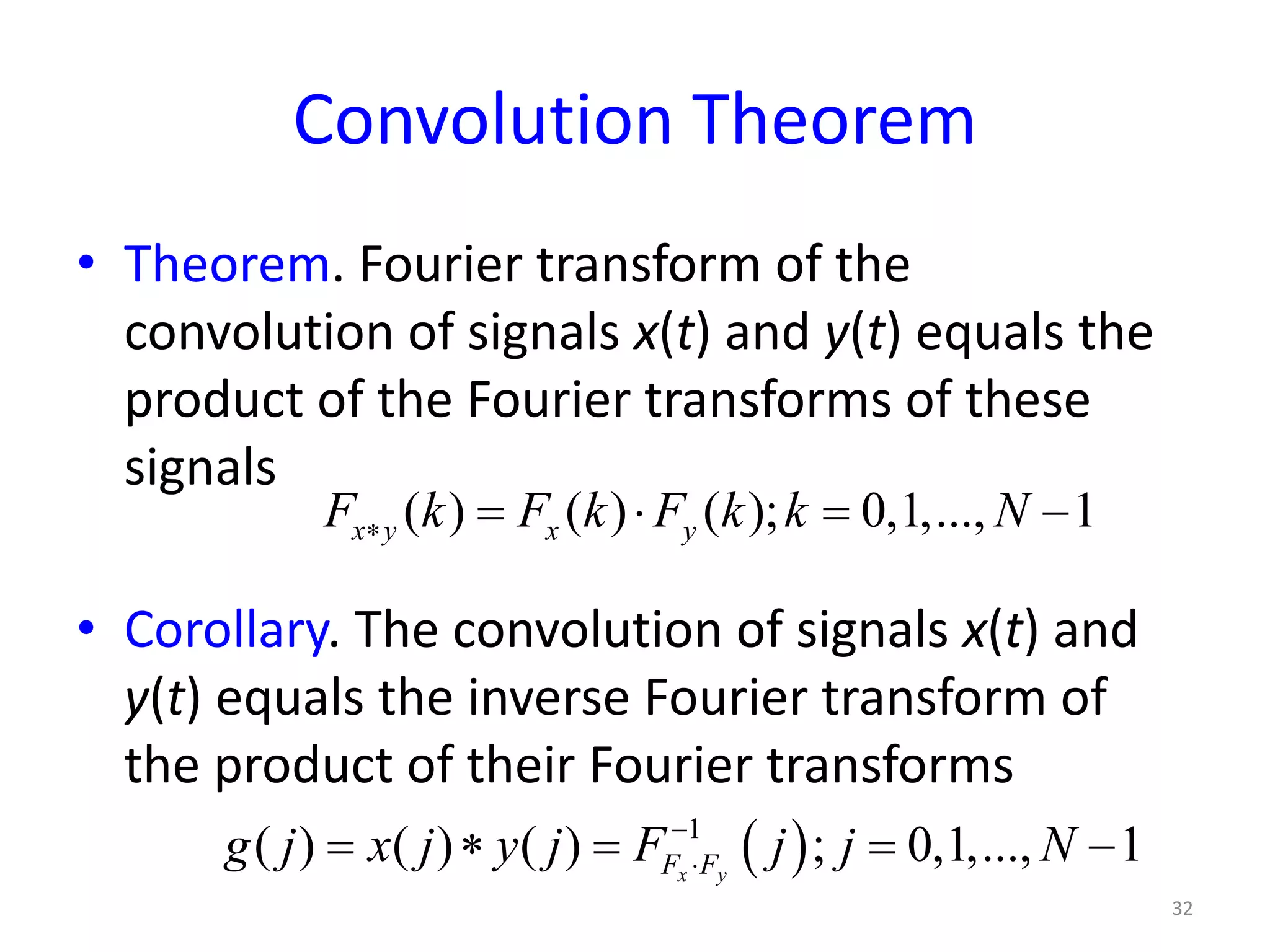
Describes convolution processes in both continuous and discrete functions and theorem relating Fourier Transform.
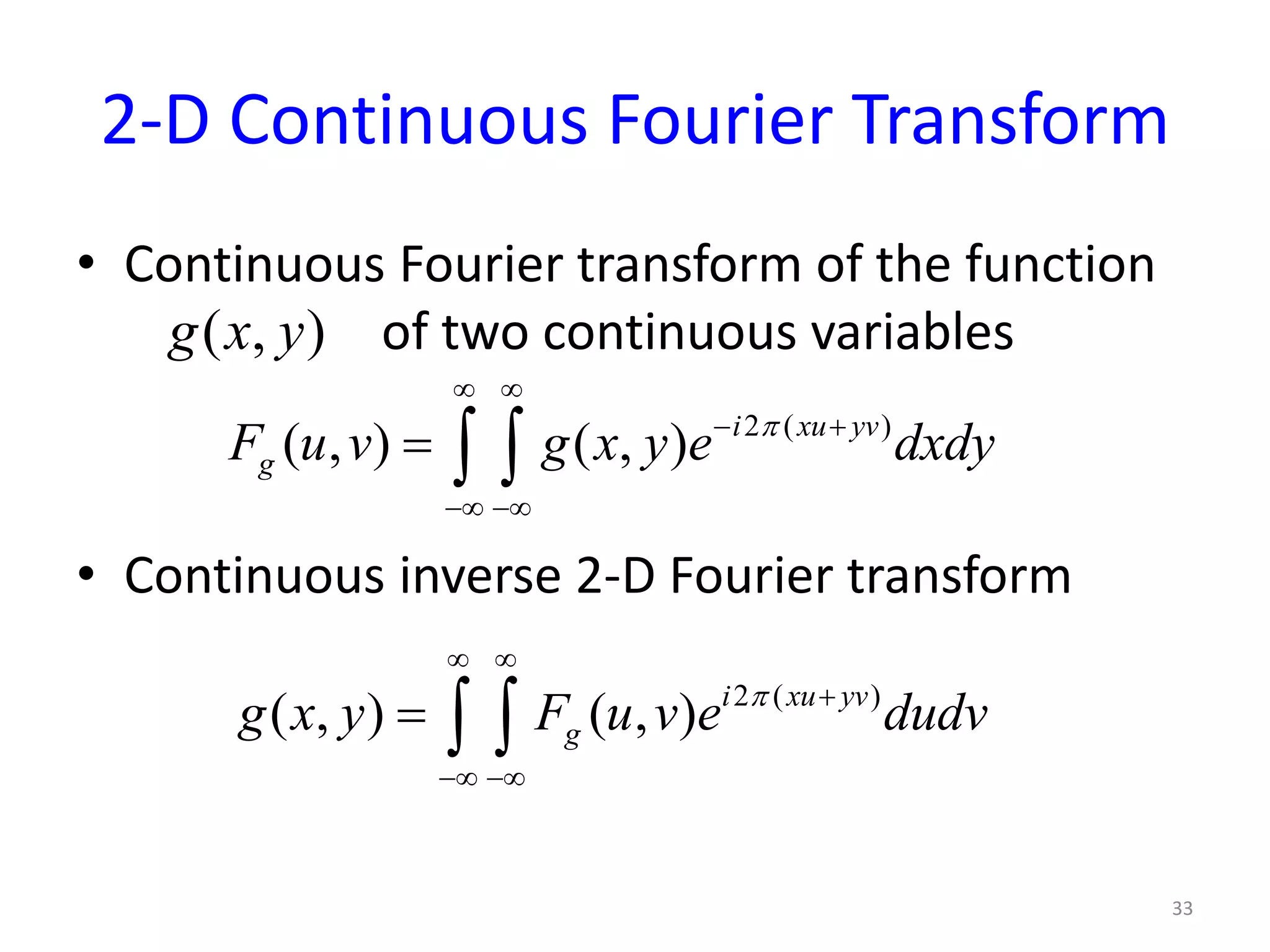
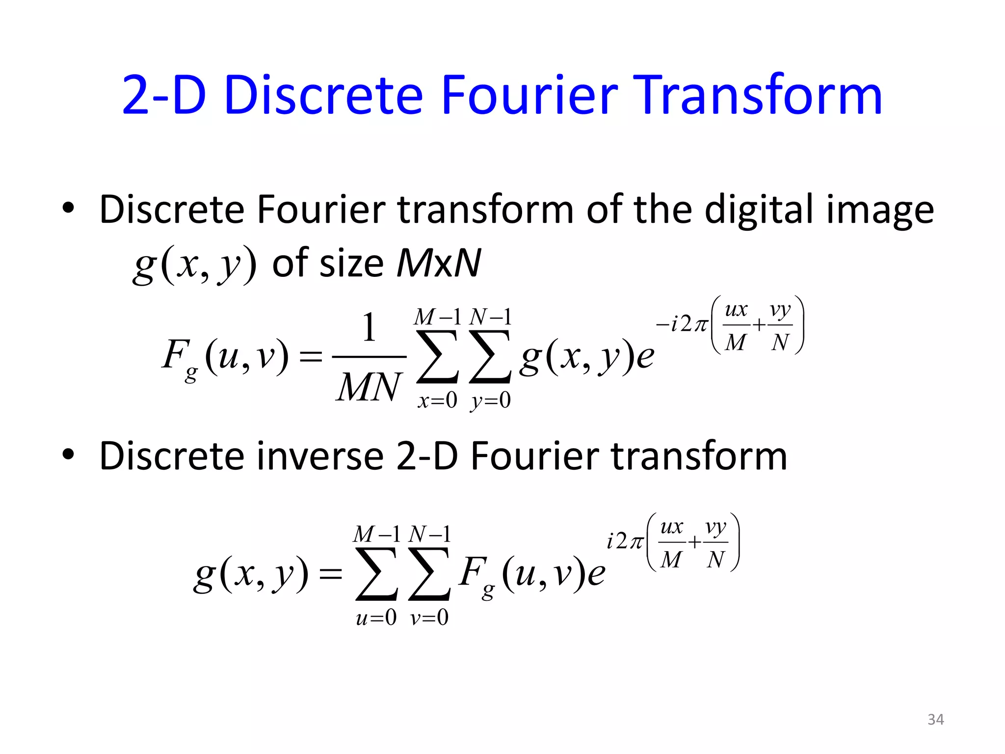
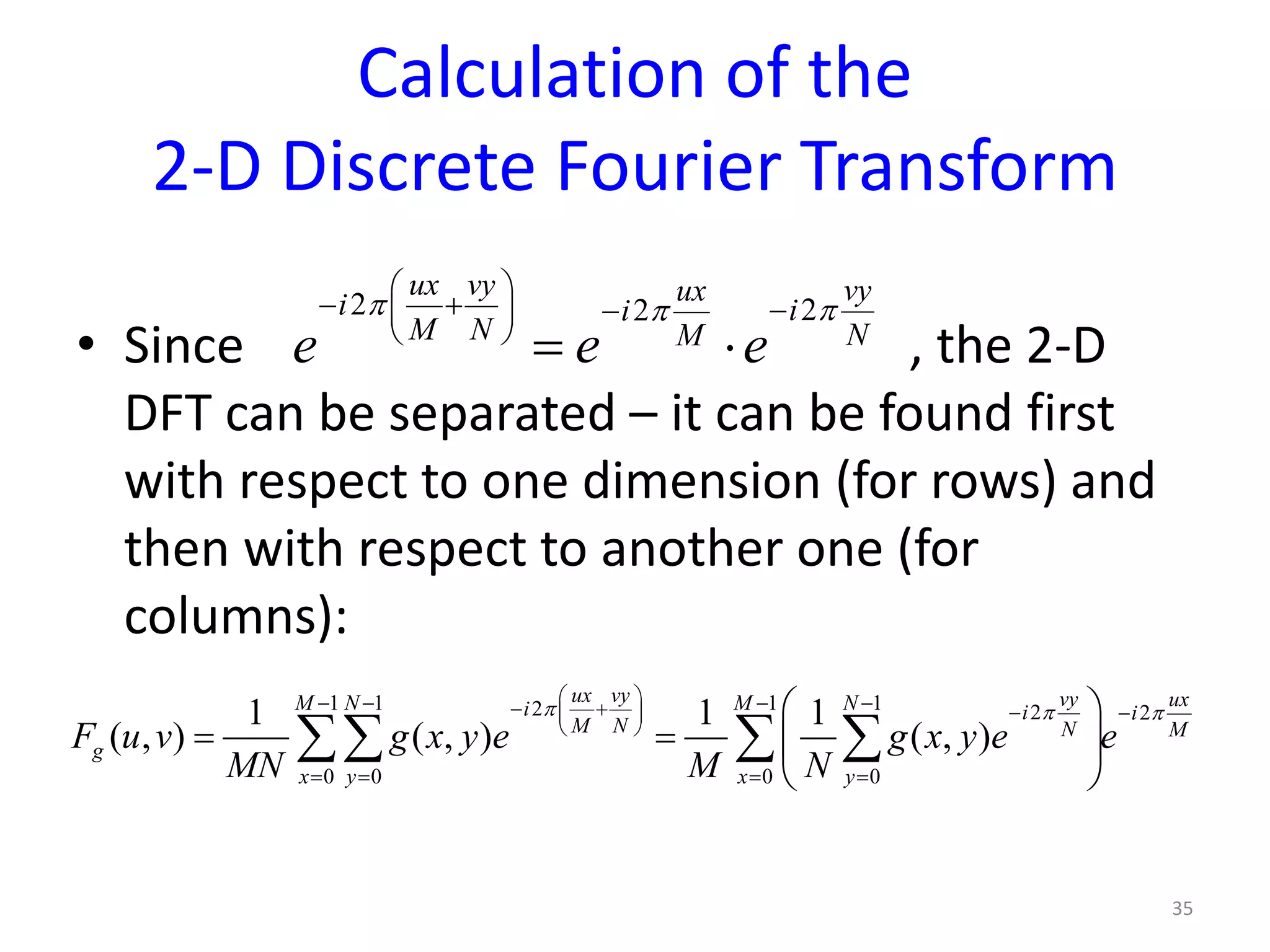
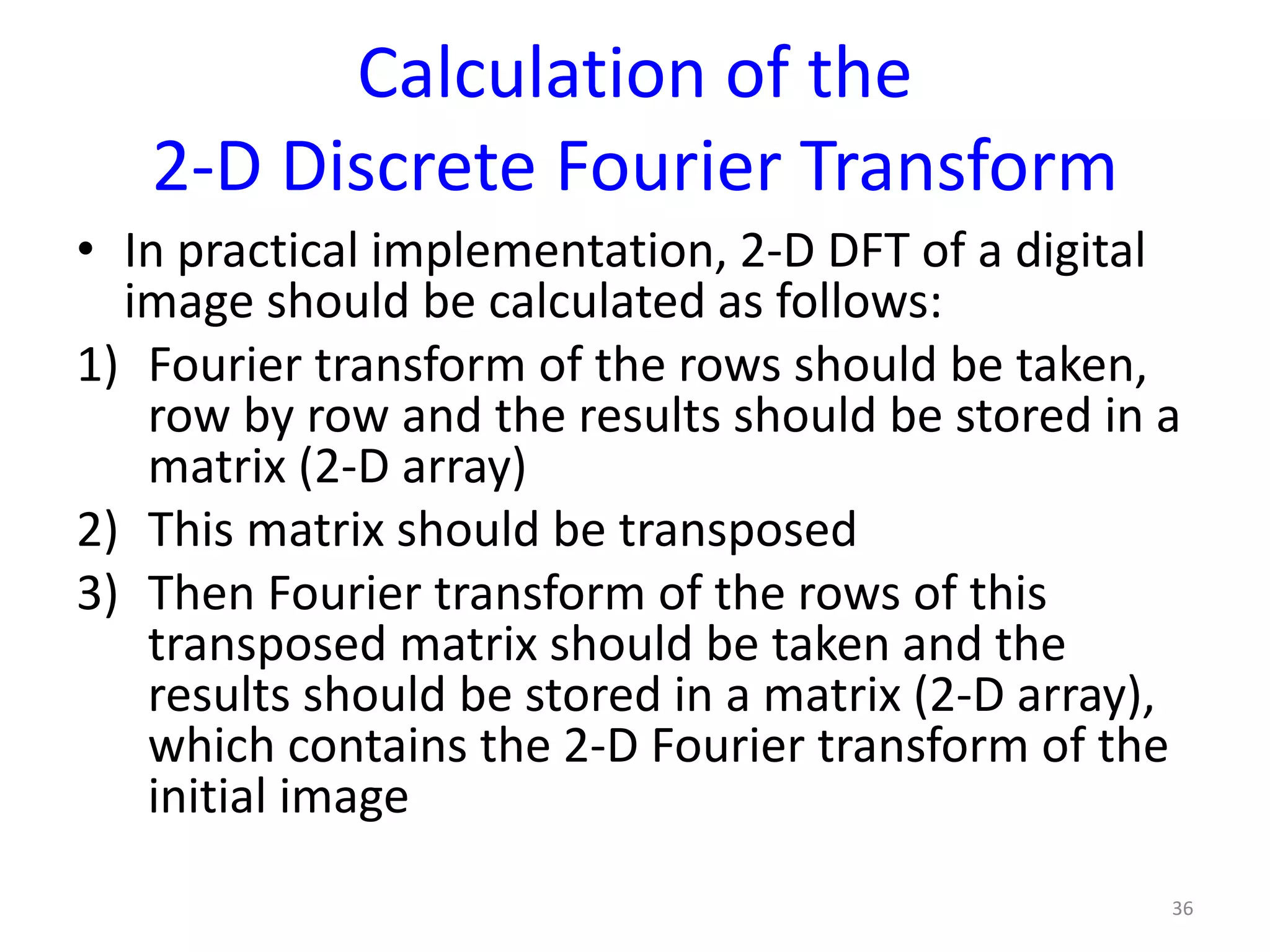
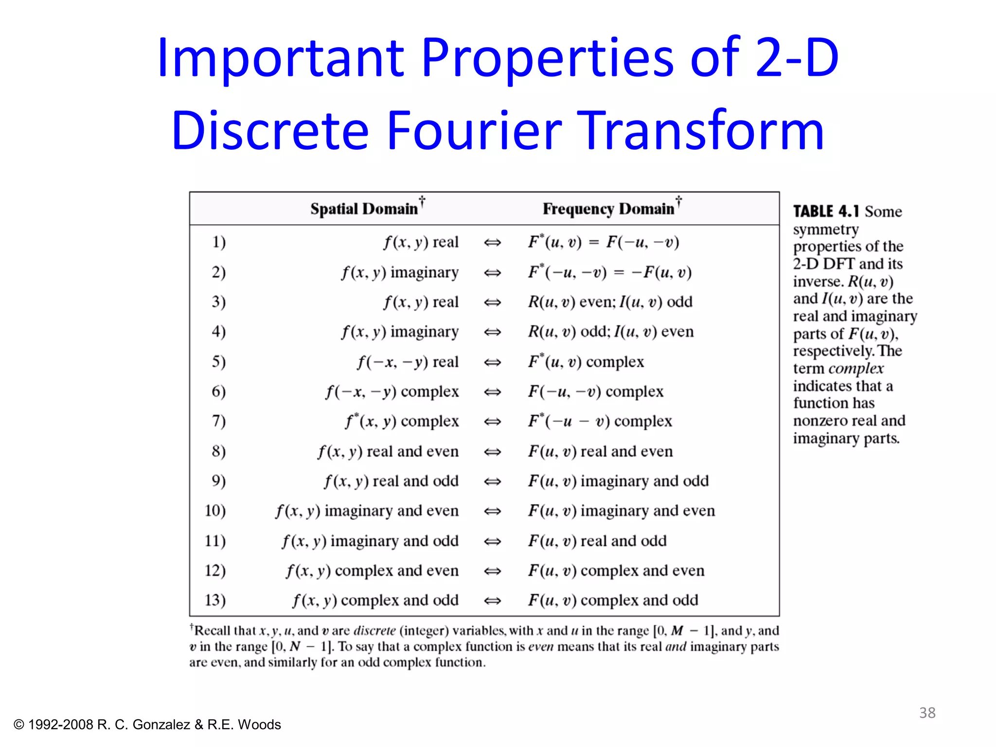
Outlines continuous and discrete 2-D Fourier Transforms and their calculation for image data processing.
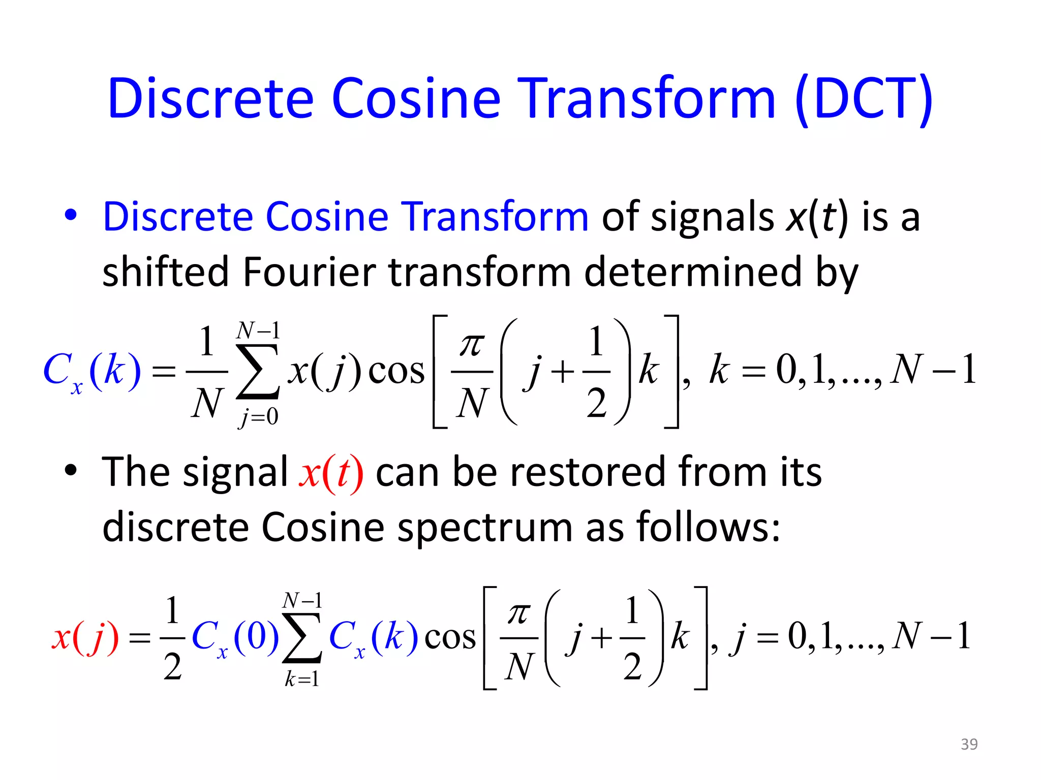
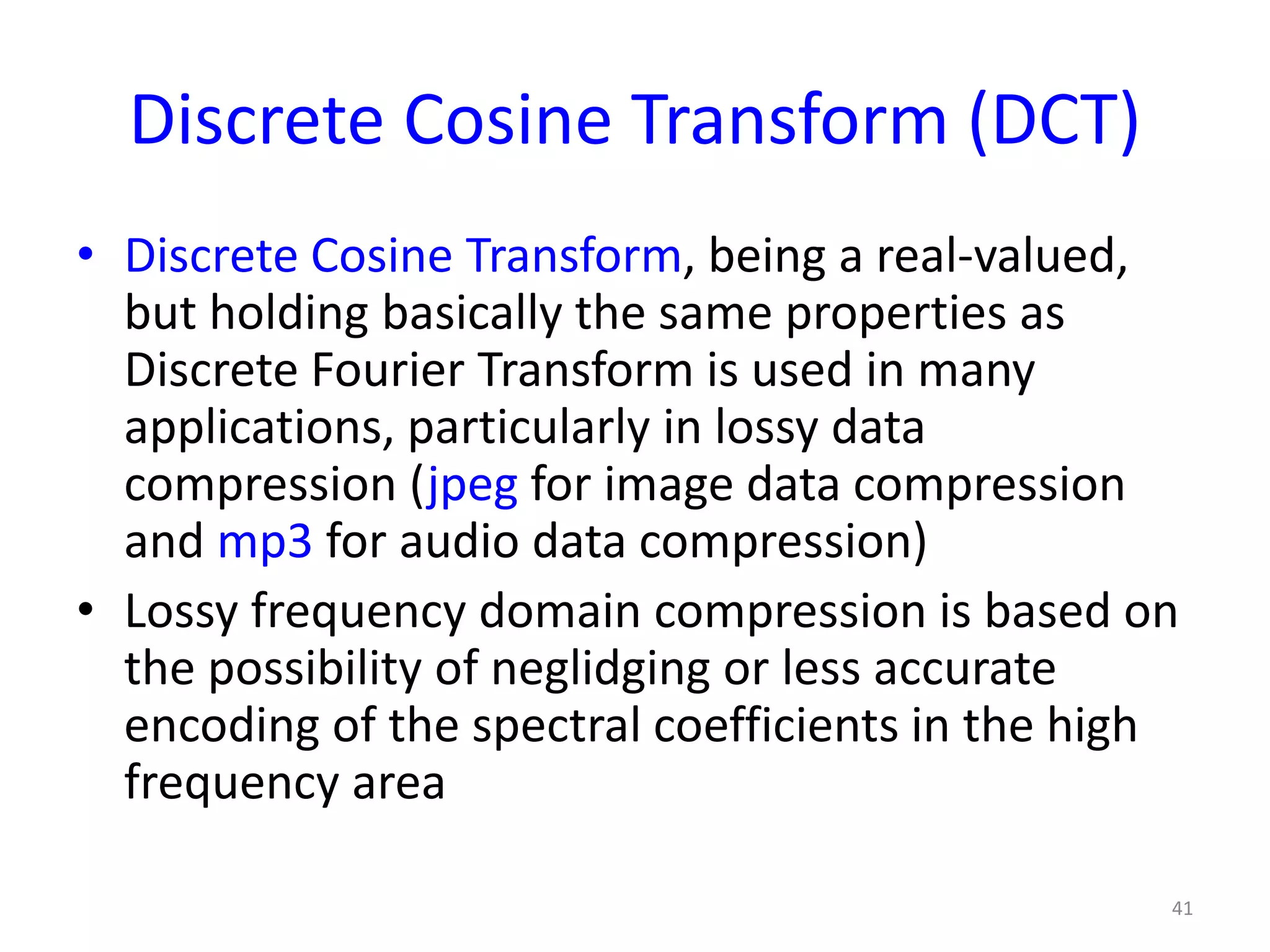
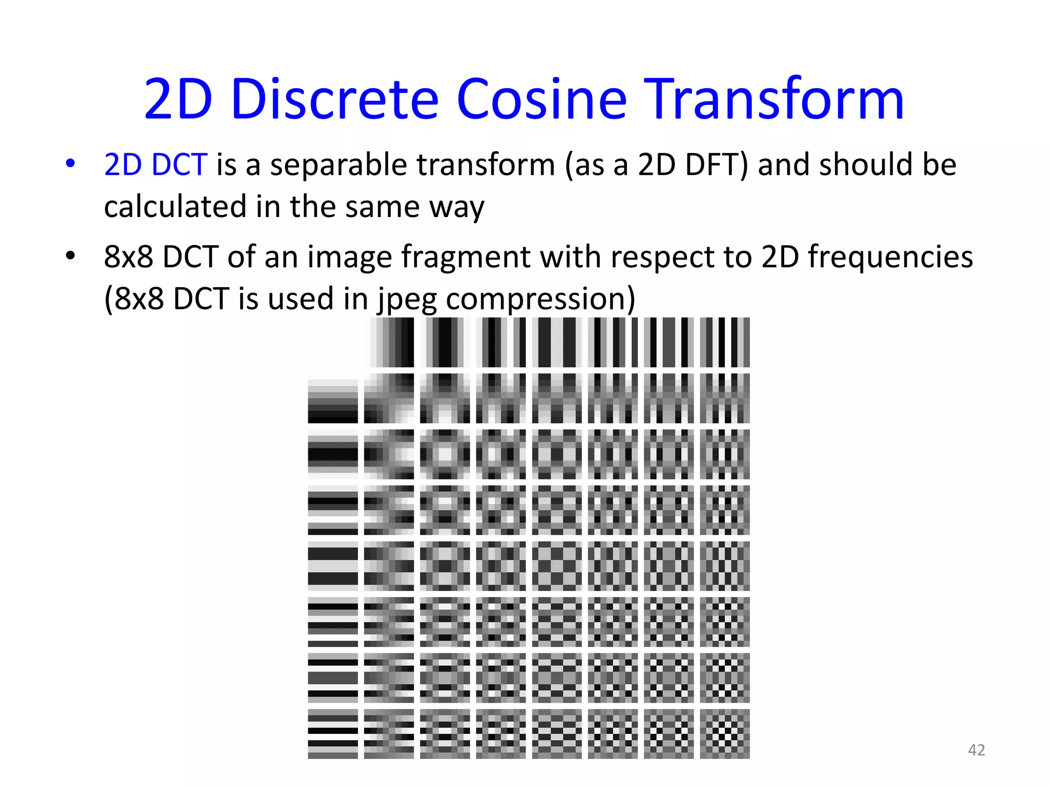
Explains DCT's properties, significance in data compression, and comparison with DFT applications.
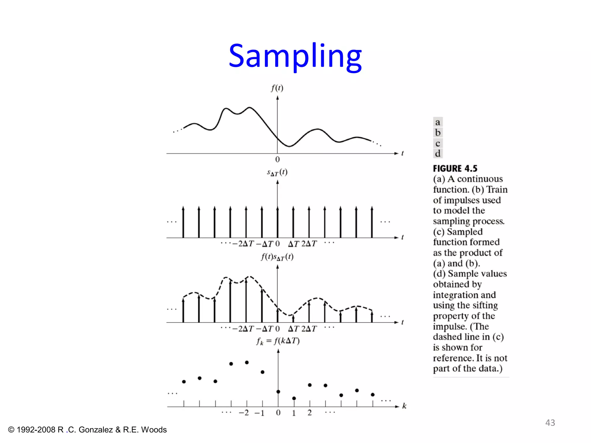
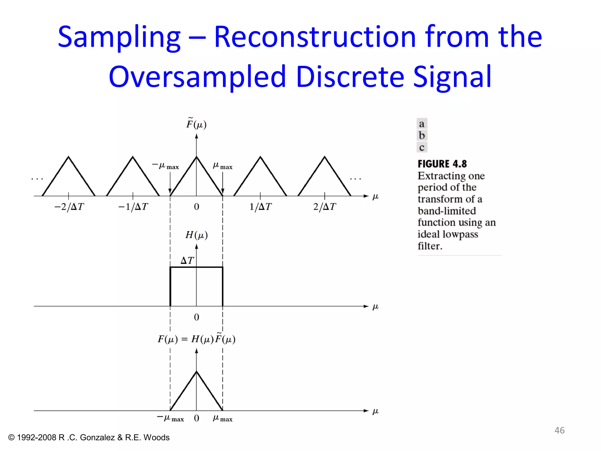
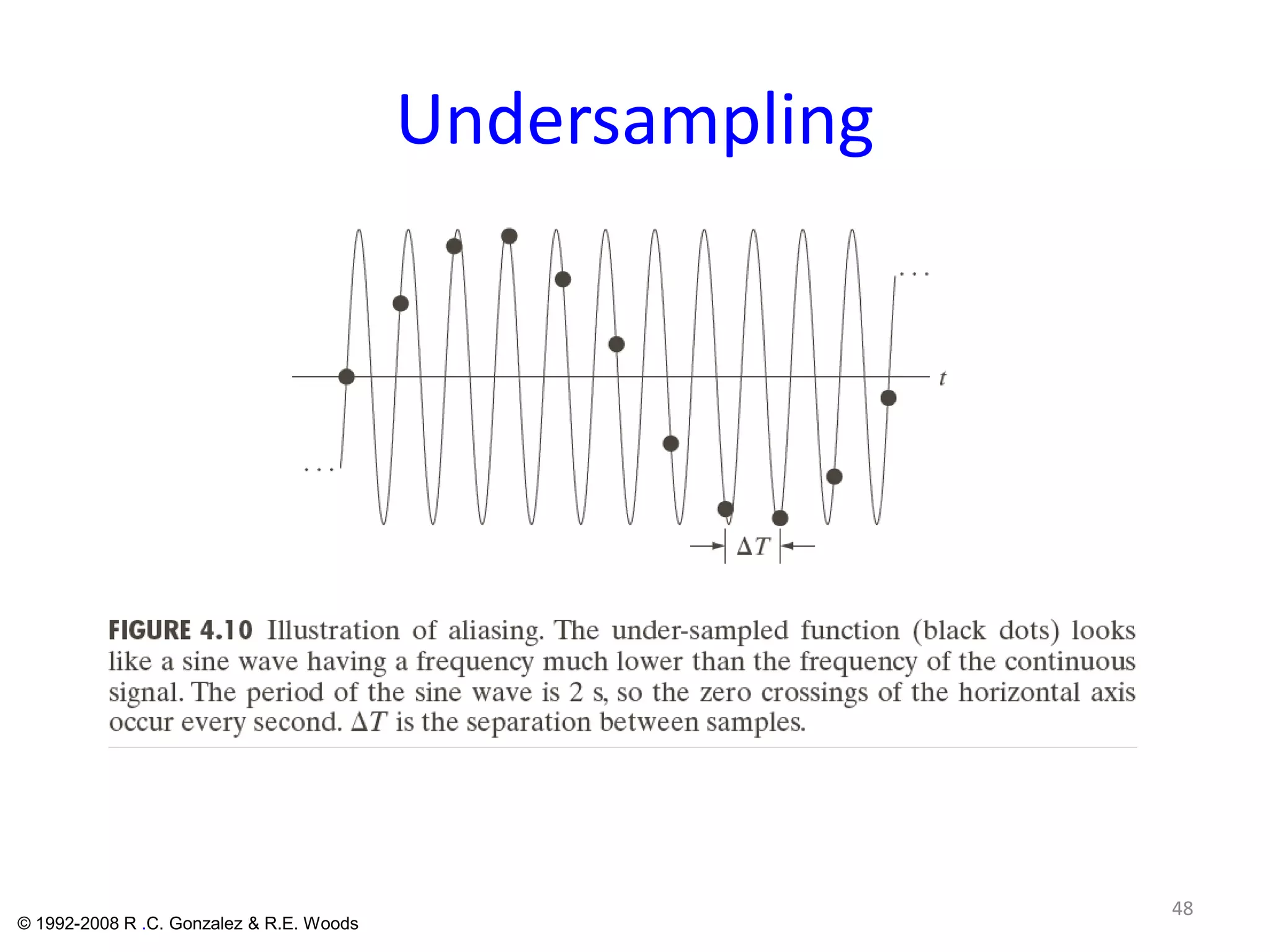
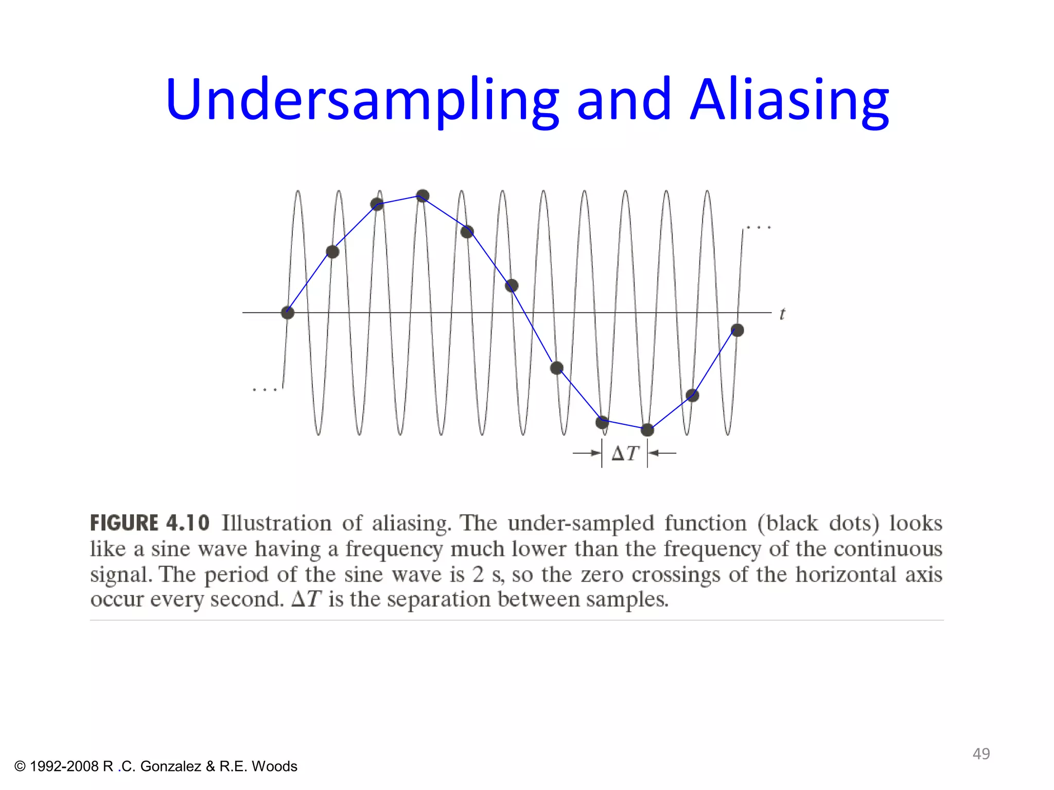
Describe sampling techniques, Nyquist rate, aliasing effects, undersampling, and reconstruction challenges.