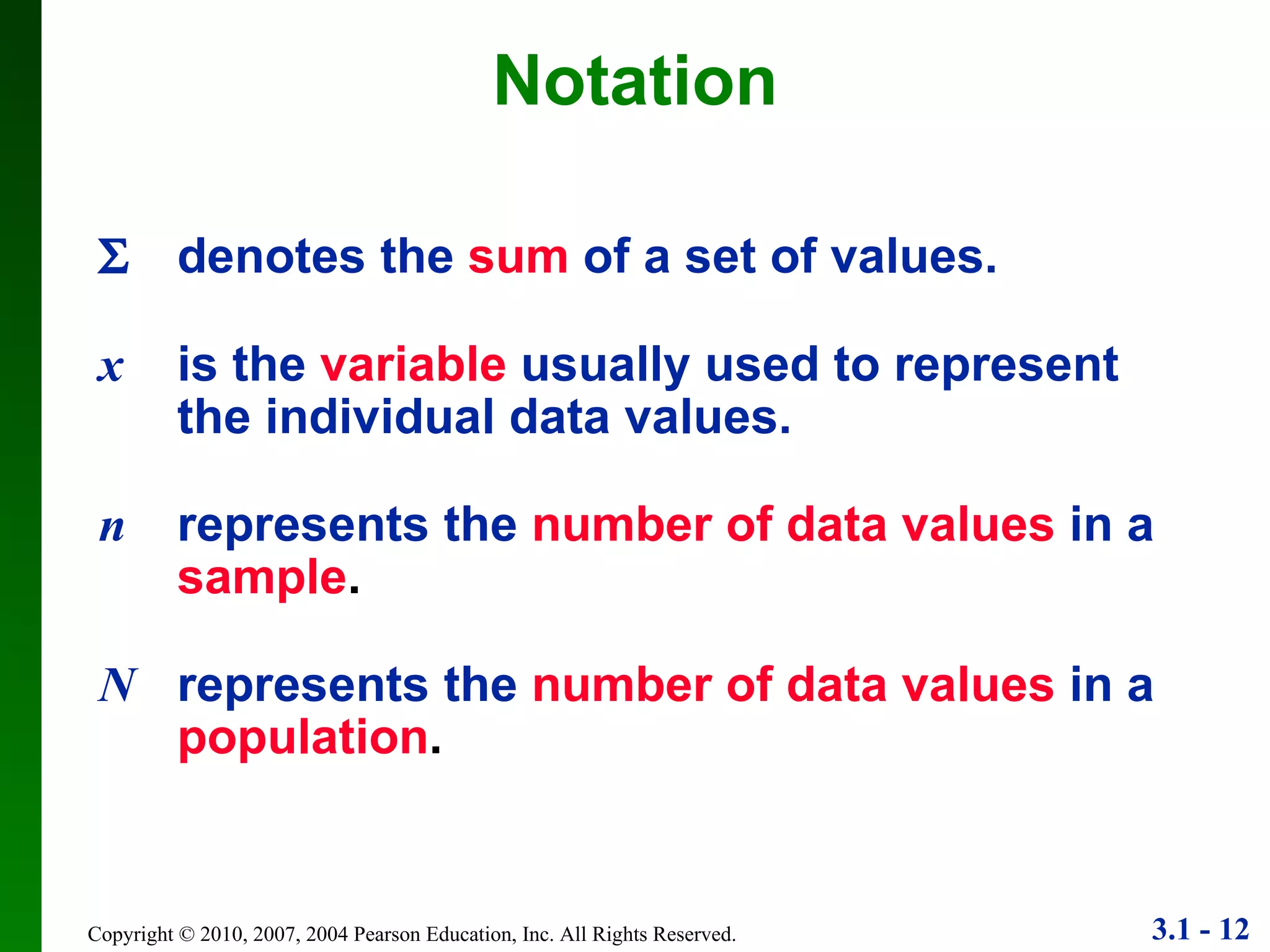
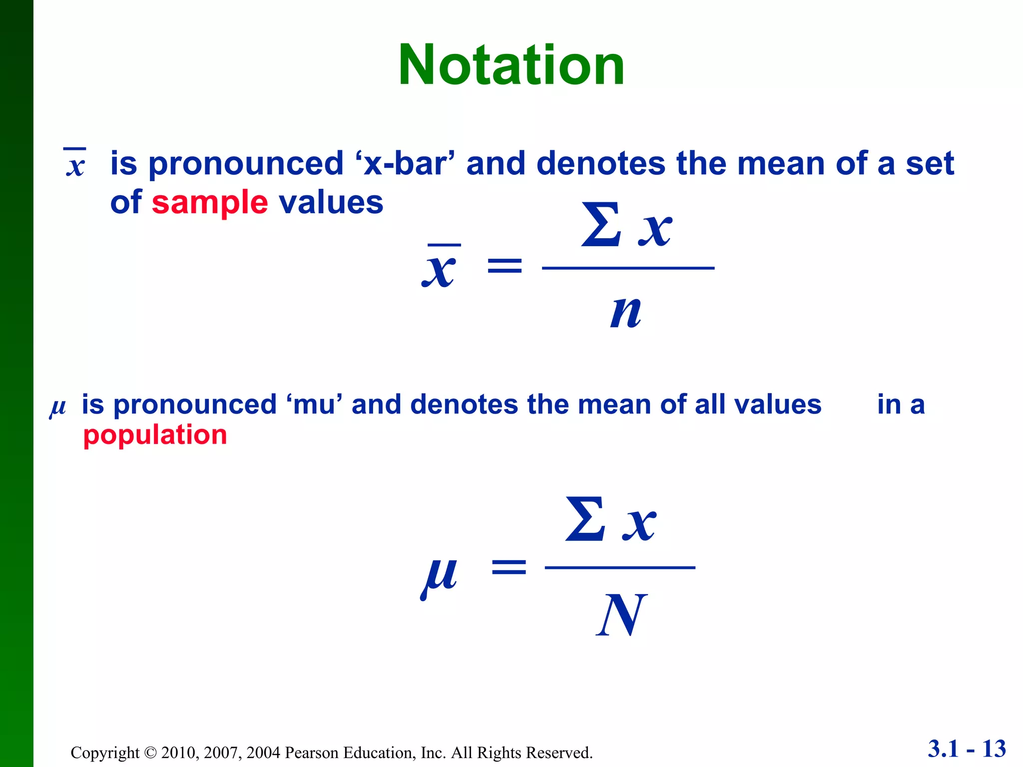
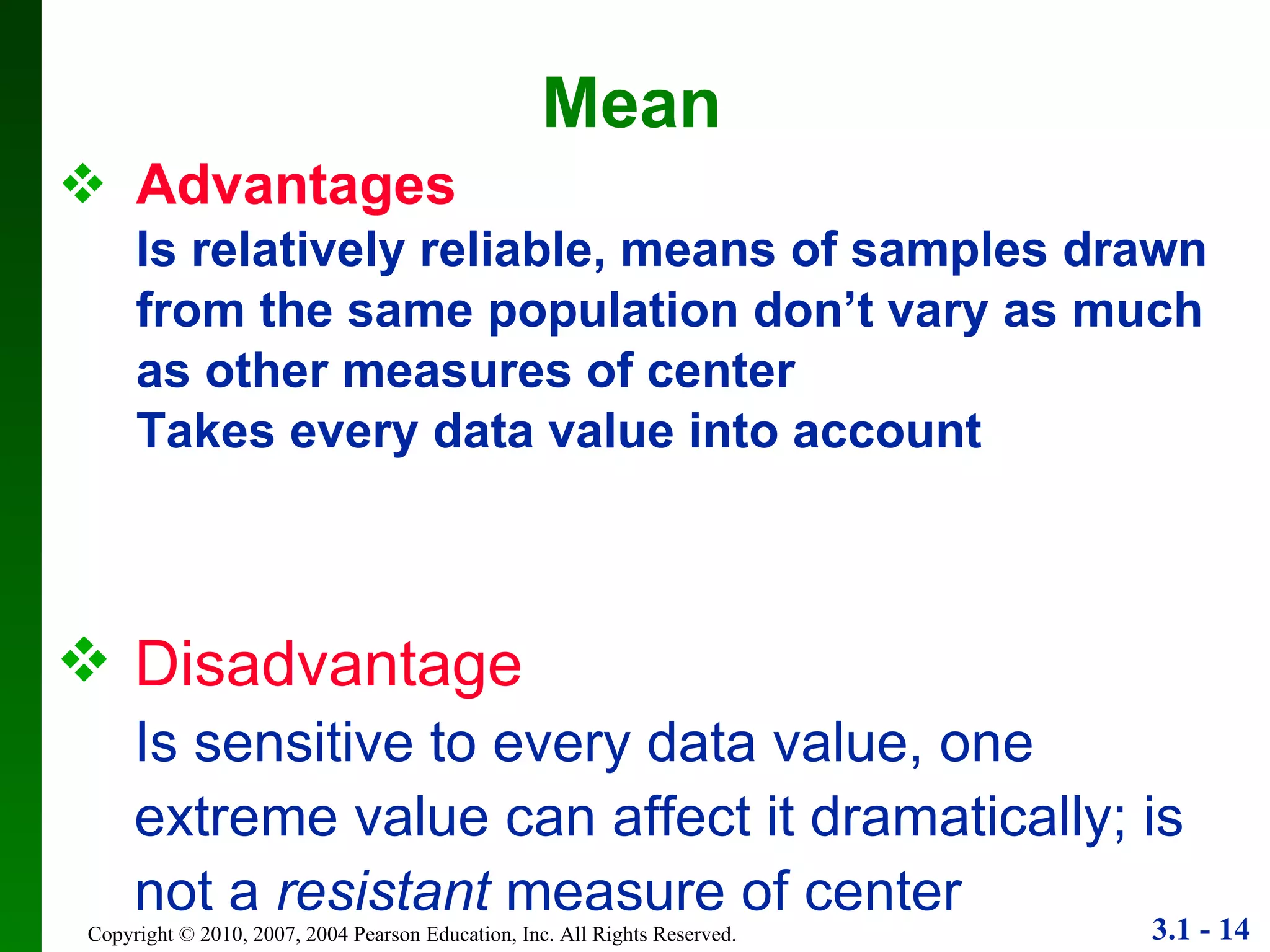
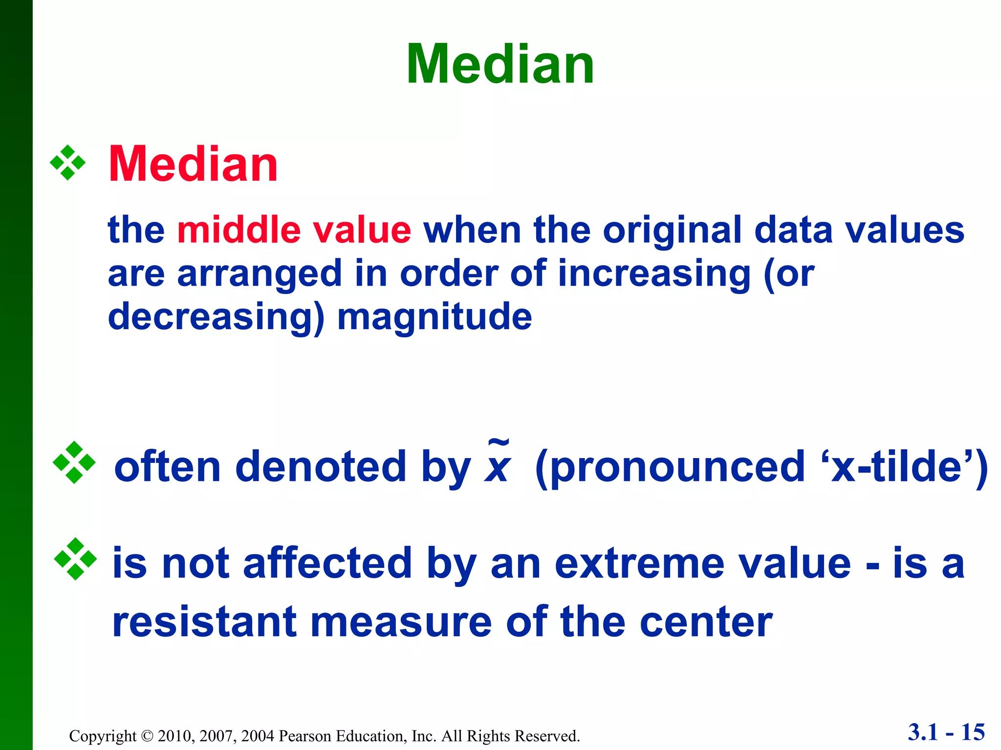
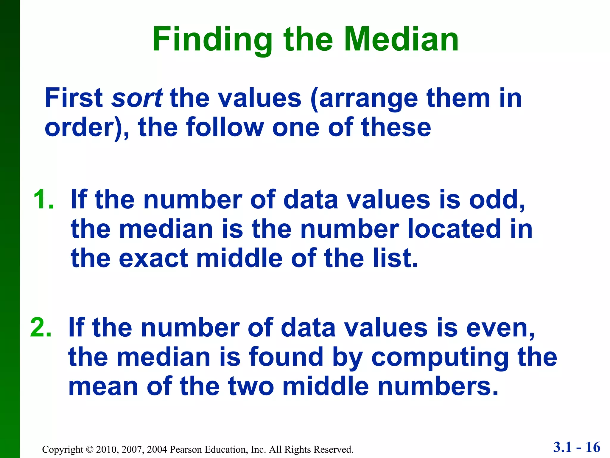
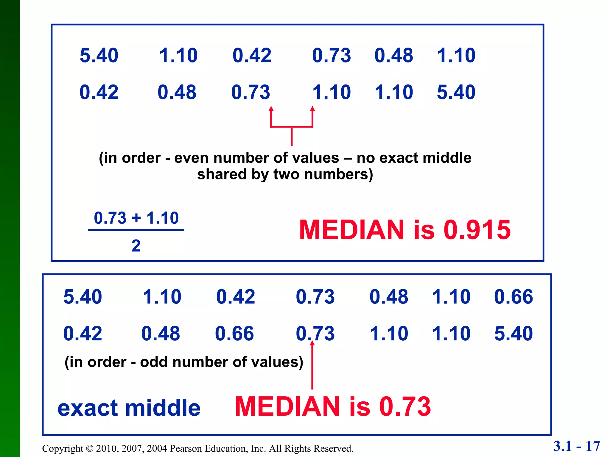
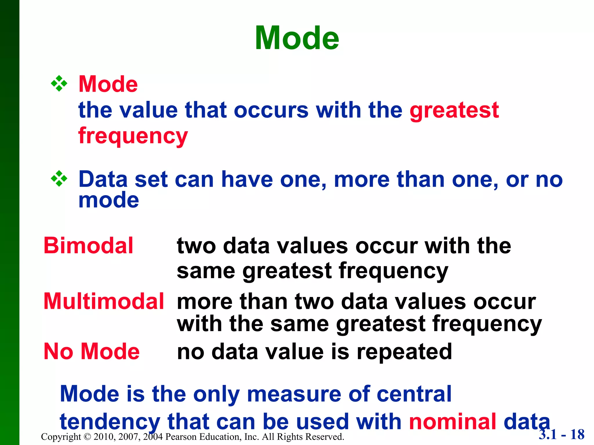
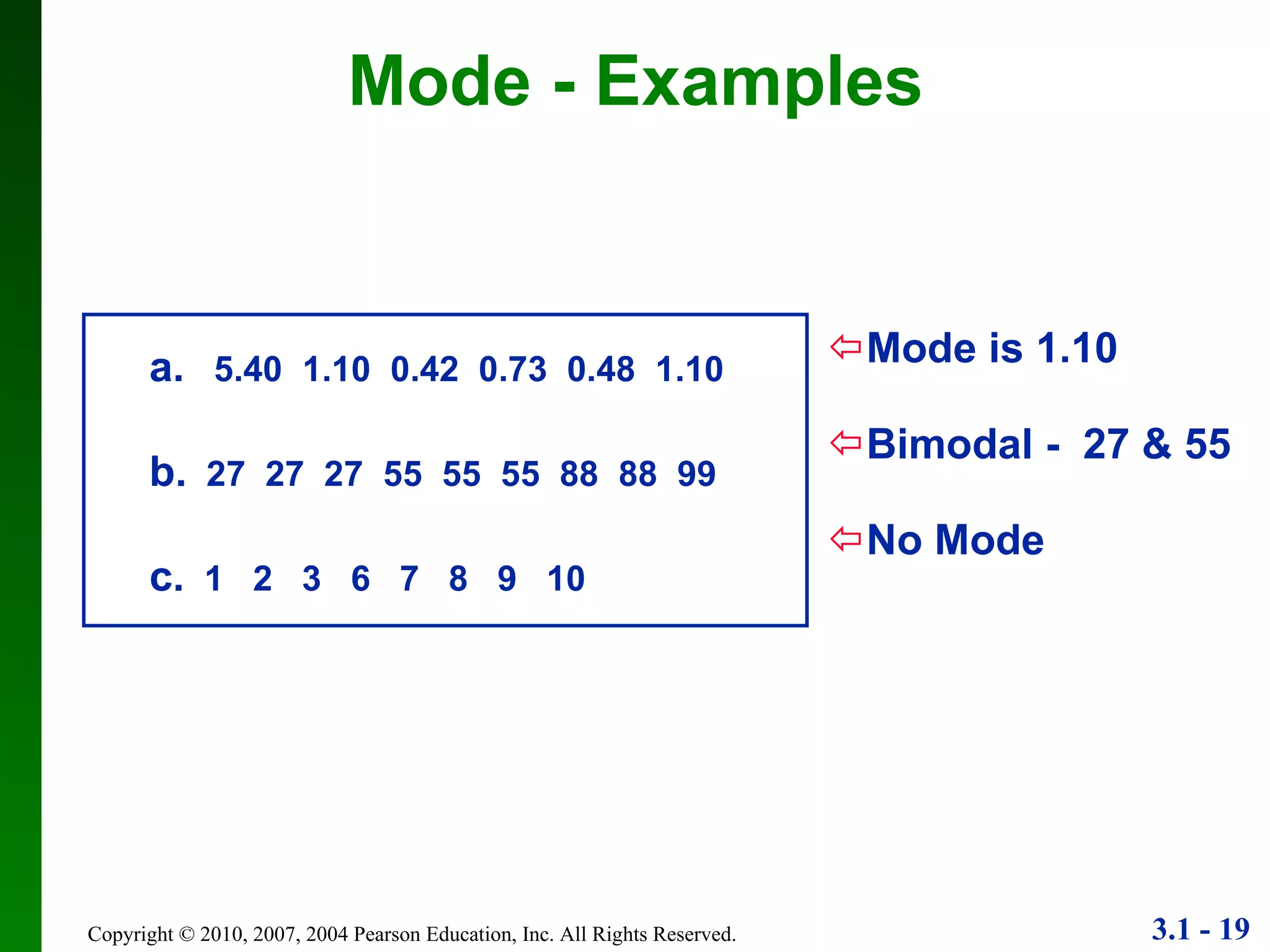
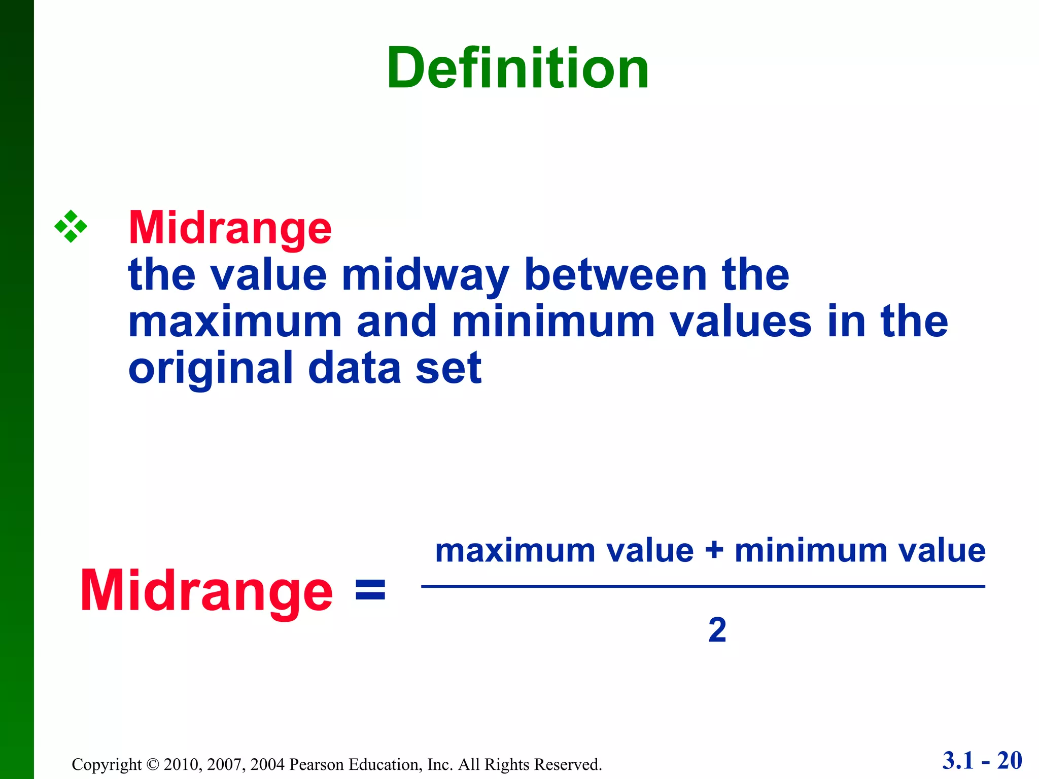
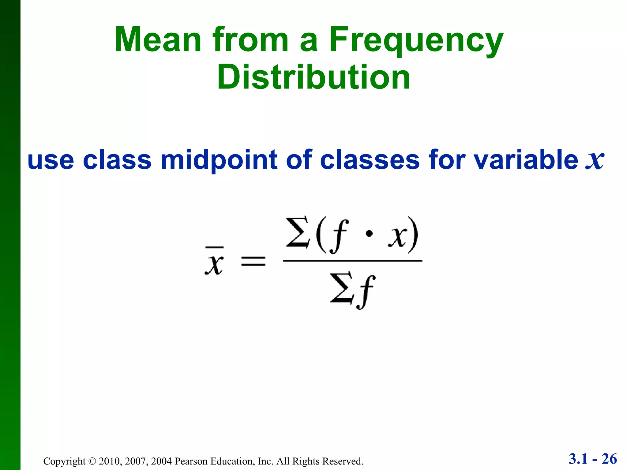
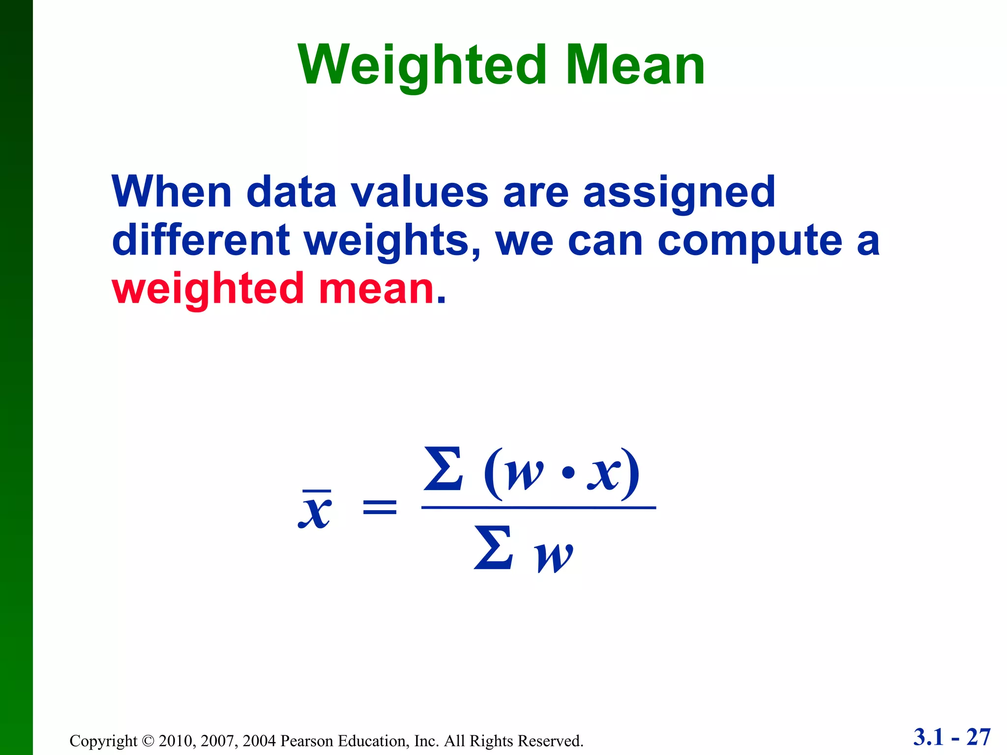
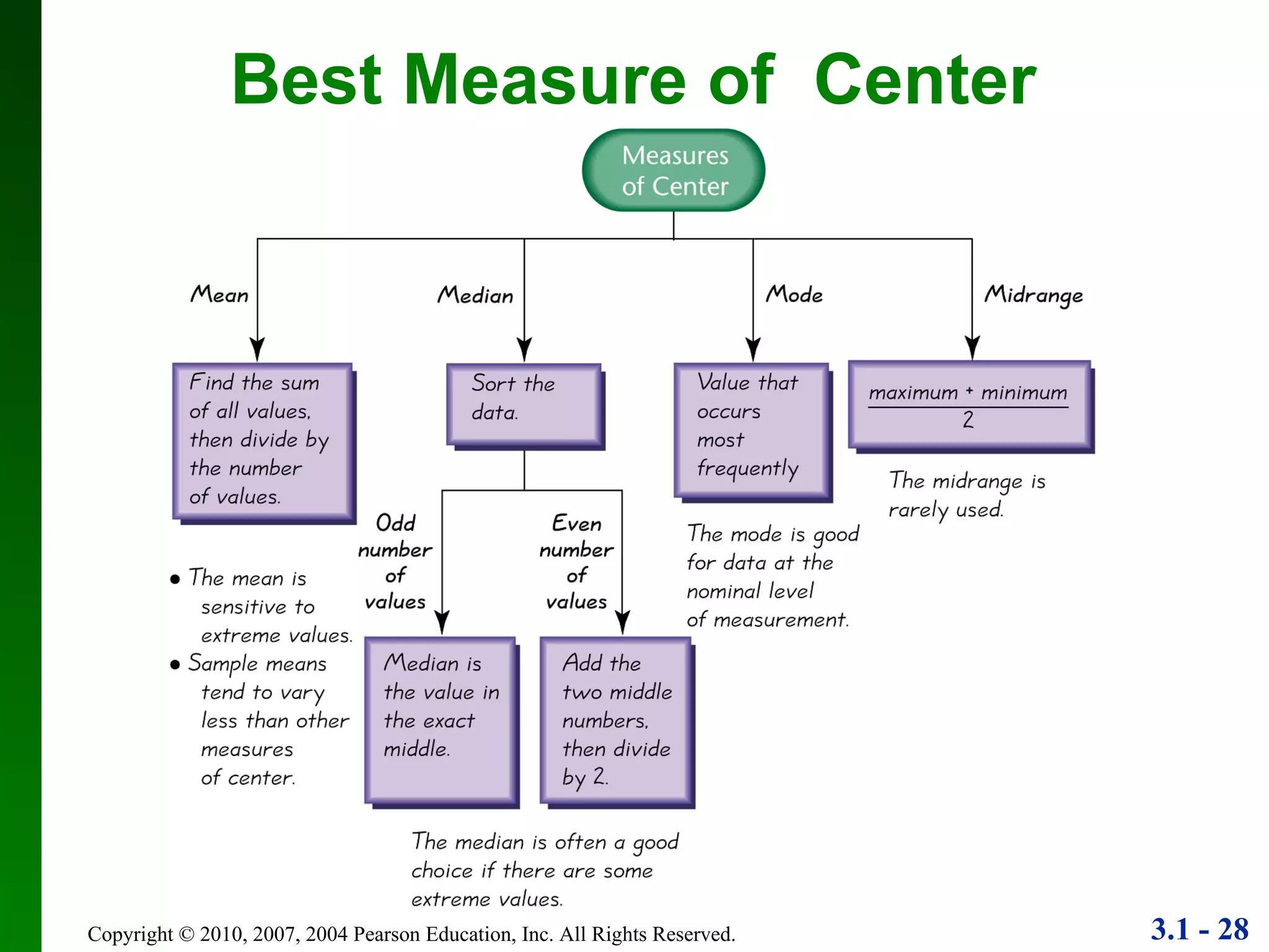
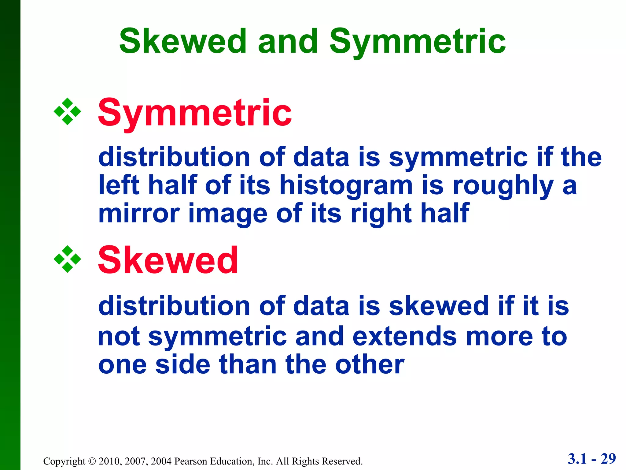
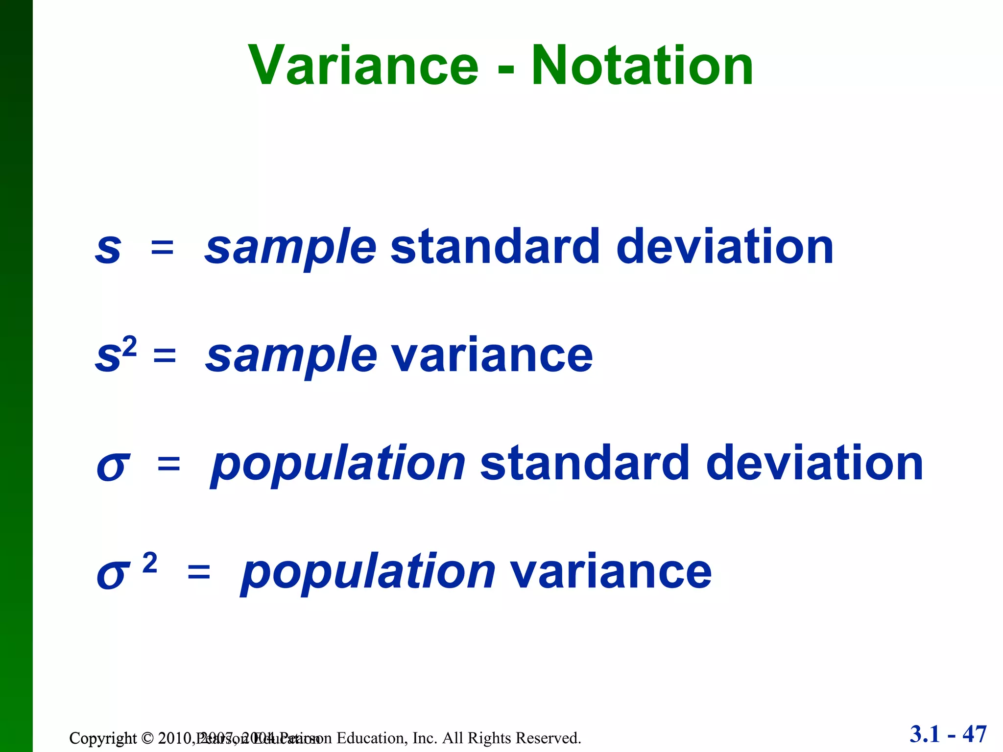
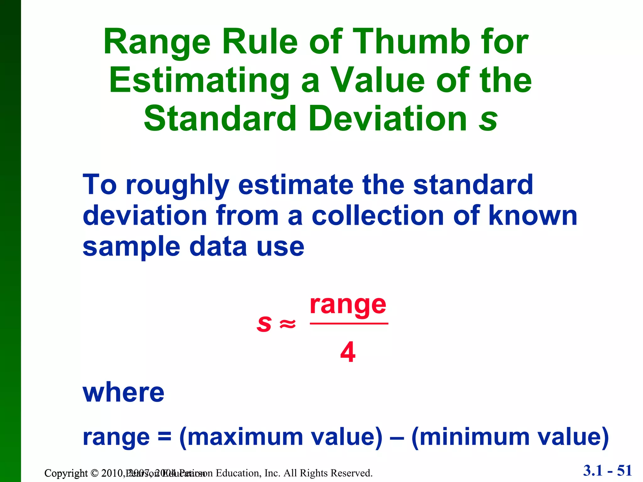
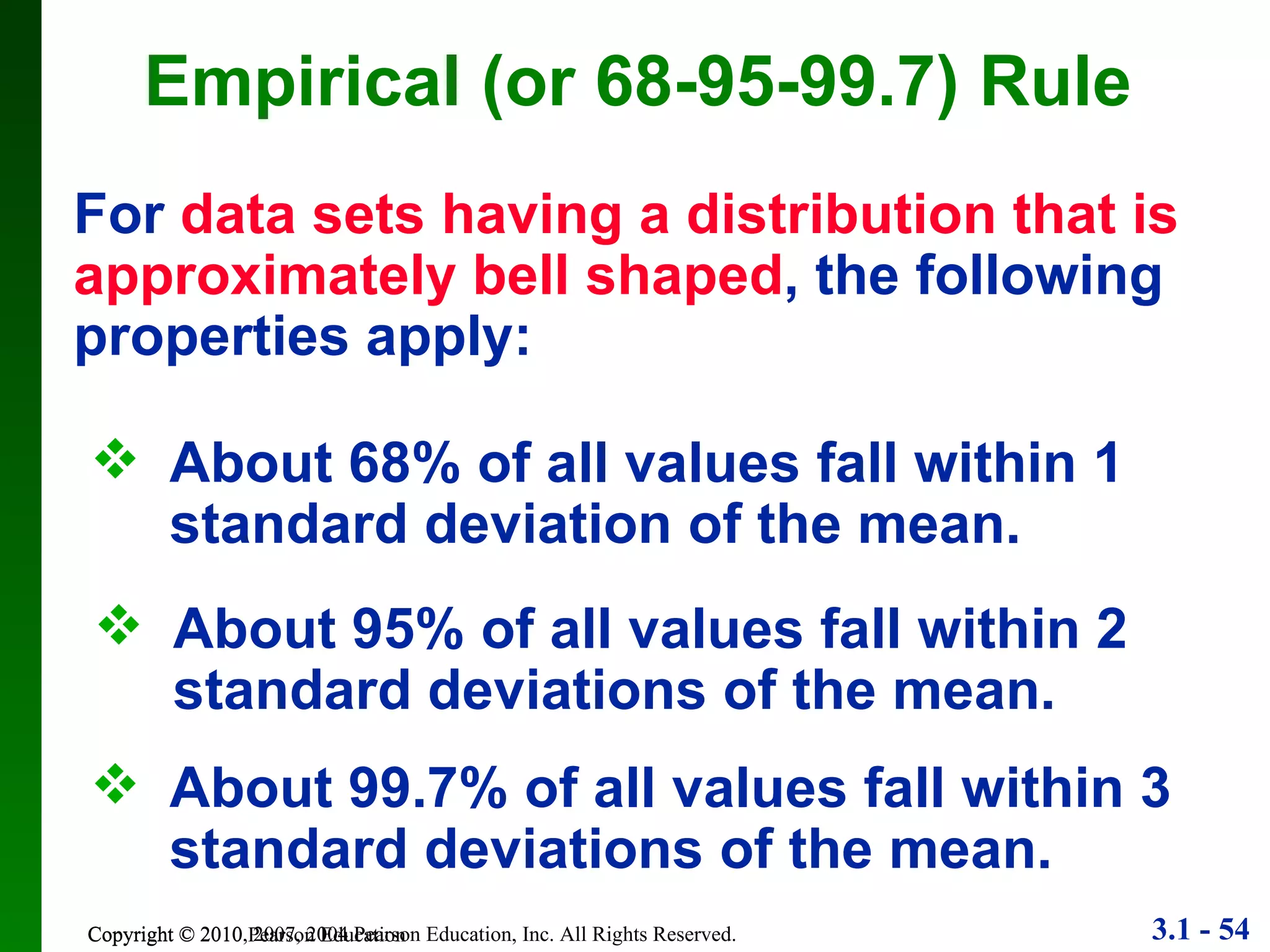
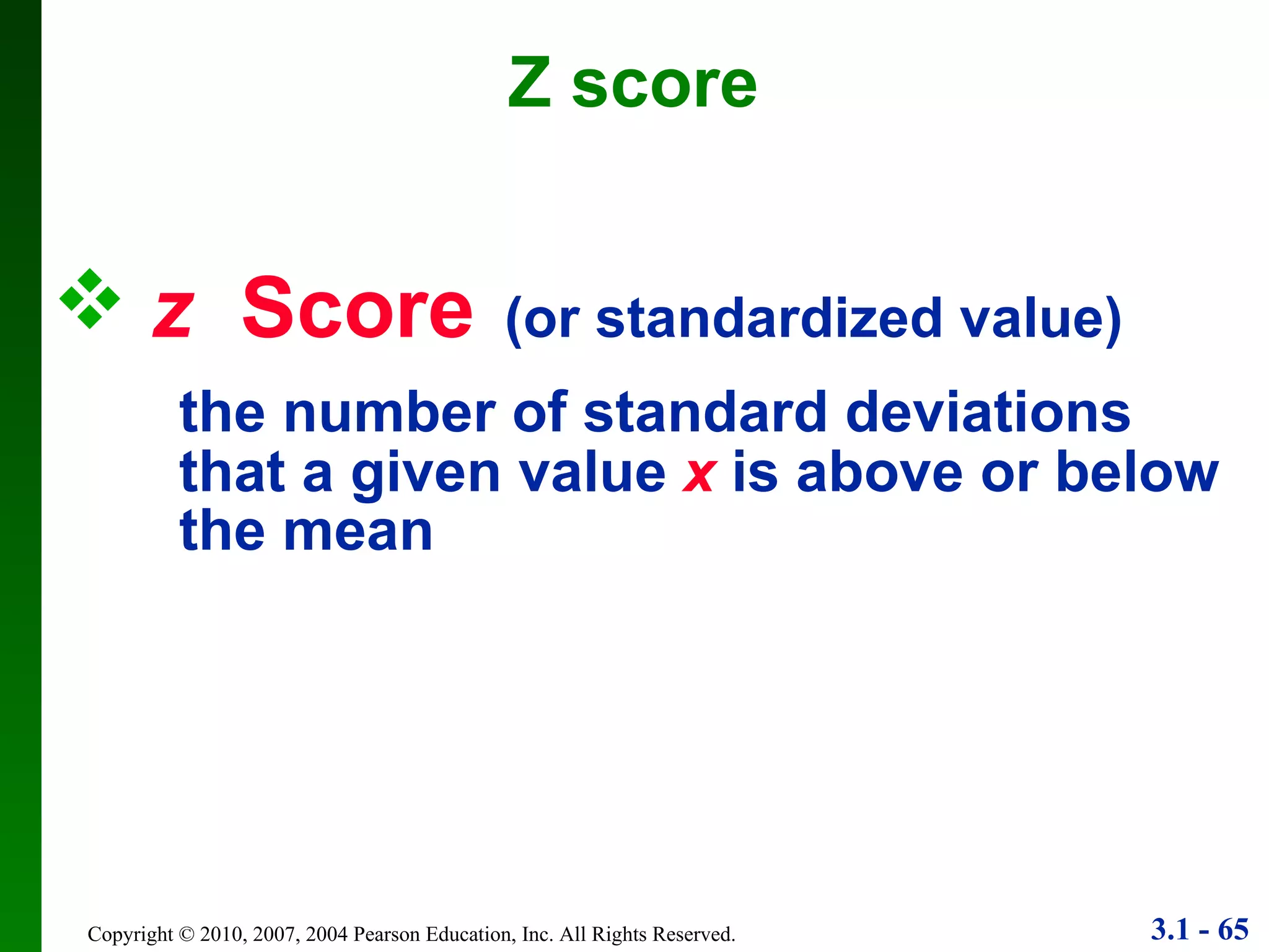
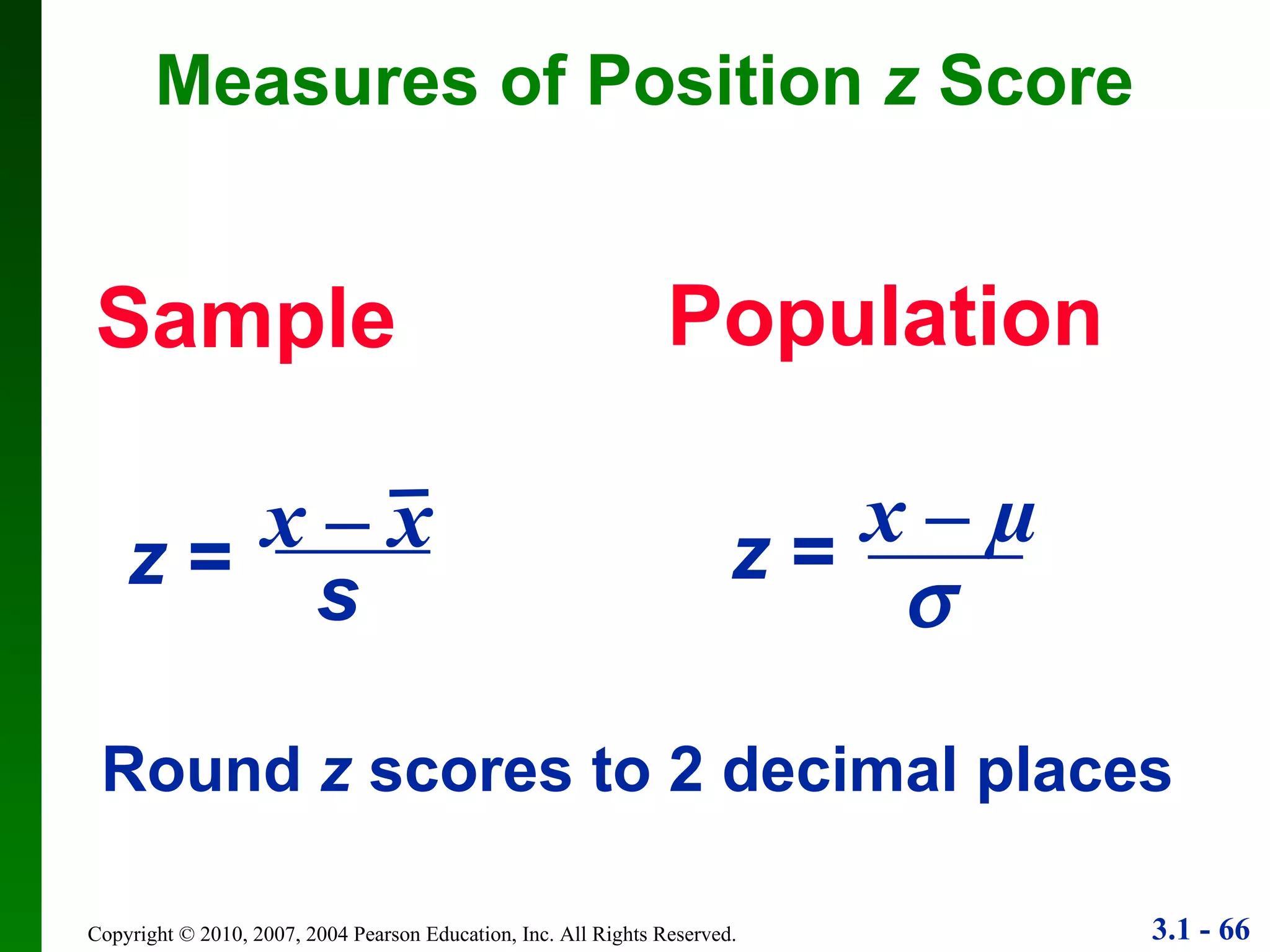
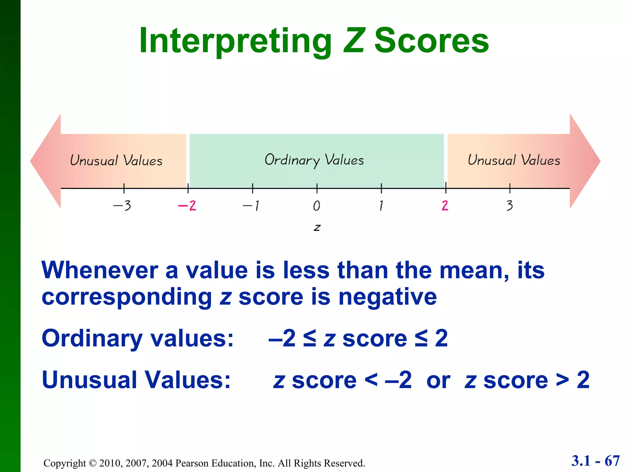
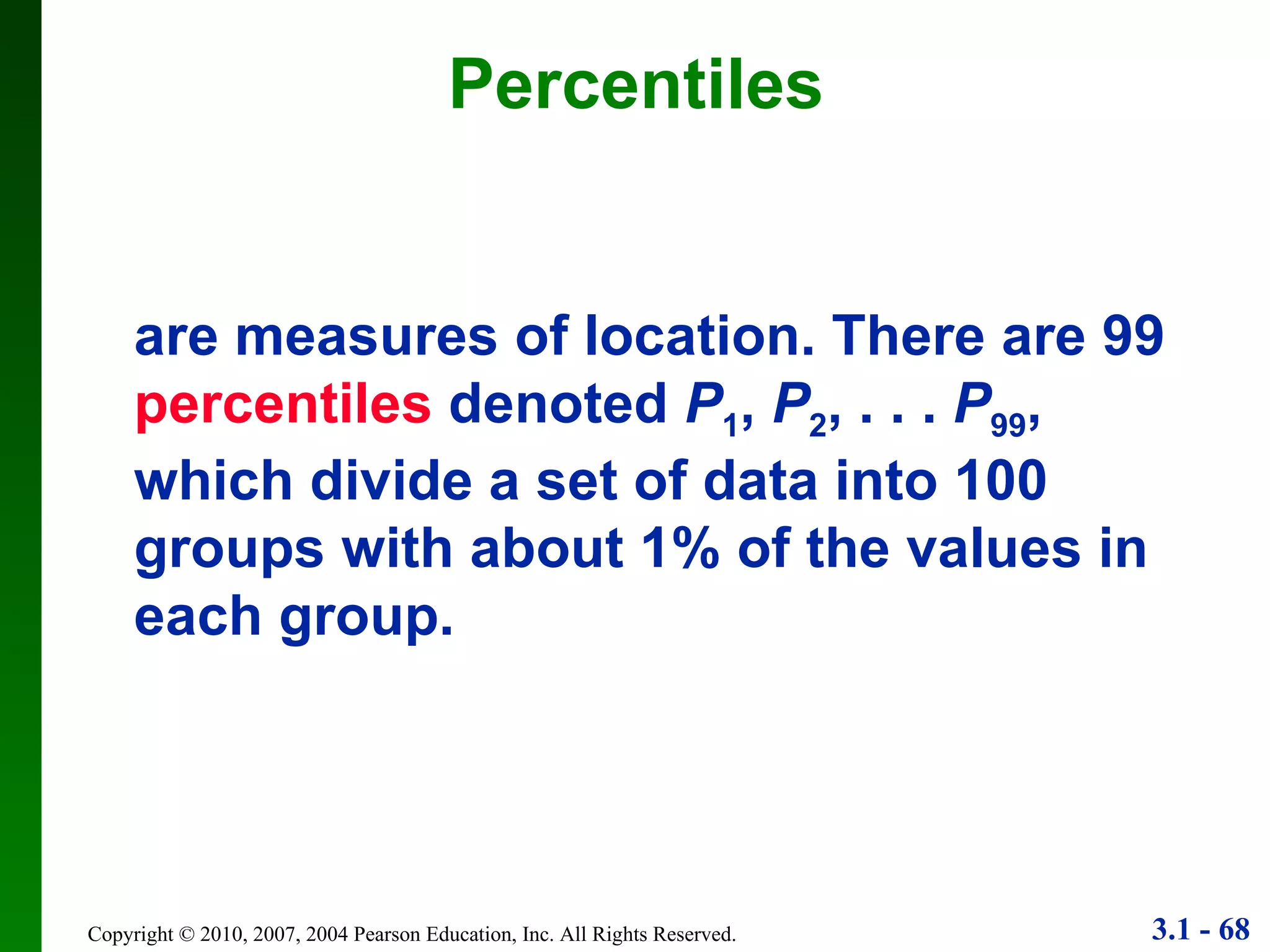
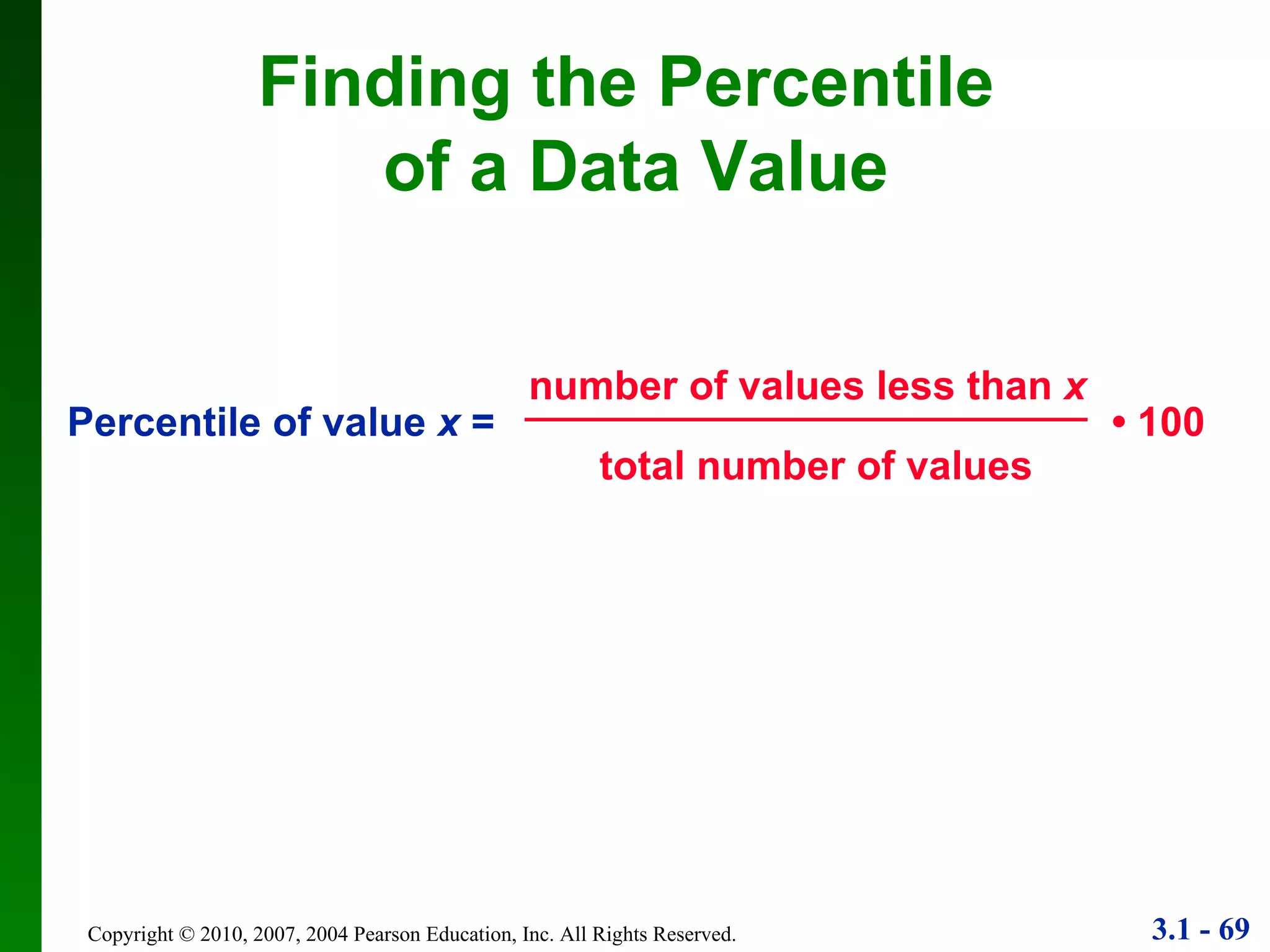
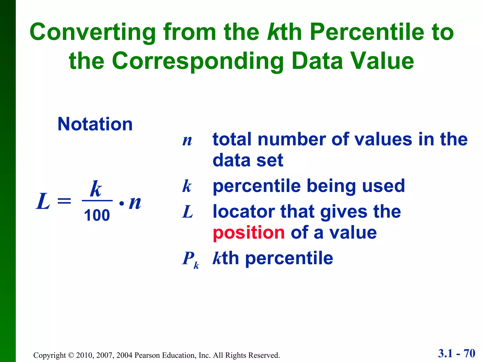
Lecture Slides  Elementary Statistics   Eleventh Edition  and the Triola Statistics Series  by Mario F. Triola
Chapter 3 Statistics for Describing, Exploring, and Comparing Data 3-1  Review and Preview 3-2  Measures of Center 3-3  Measures of Variation 3-4  Measures of Relative Standing and Boxplots
Created by Tom Wegleitner, Centreville, Virginia Section 3-1  Review and Preview
Chapter 1 Distinguish between population and sample, parameter and statistic Good sampling methods:  simple random sample , collect in appropriate ways  Chapter 2 Frequency distribution: summarizing data Graphs designed to help understand data Center, variation, distribution, outliers, changing characteristics over time Review
Important Statistics  Mean, median, standard deviation, variance   Understanding and Interpreting   these important statistics Preview
Descriptive Statistics  In this chapter we’ll learn to   summarize or  describe   the important  characteristics of a known set of data   Inferential Statistics   In later chapters we’ll learn to   use sample data to make   inferences or generalizations   about a population Preview
Section 3-2 Measures of Center
Key Concept Characteristics of center. Measures of center, including mean and median, as tools for analyzing data. Not only determine the value of each measure of center, but also interpret those values.
Basics Concepts of Measures of Center Part 1
Measure of Center Measure of Center the value at the center or middle of a  data set
Arithmetic Mean Arithmetic Mean (Mean) the measure of center obtained by adding the values and dividing the total by the number of values What most people call an  average .
Notation    denotes the  sum  of a set of values. x   is the  variable  usually used to represent the individual data values. n   represents the  number of data values  in a  sample . N represents the  number of data values  in a  population .
µ   is pronounced ‘mu’ and denotes the   mean of all values   in a  population Notation is pronounced ‘x-bar’ and denotes the mean of a set of  sample  values x   = n    x x   N µ   =    x
Advantages Is relatively reliable, means of samples drawn from the same population don’t vary as much as other measures of center Takes every data value into account Mean Disadvantage Is sensitive to every data value, one extreme value can affect it dramatically; is not a  resistant  measure of center
Median the  middle value  when the original data values are arranged in order of increasing (or decreasing) magnitude Median is not affected by an extreme value - is a resistant measure of the center often denoted by  x   (pronounced ‘x-tilde’) ~
Finding the Median 1. If the number of data values is odd, the median is the number located in the exact middle of the list. 2. If the number of data values is even, the median is found by computing the mean of the two middle numbers. First  sort  the values (arrange them in order), the follow one of these
5.40  1.10  0.42 0.73  0.48  1.10  0.66  0.42   0.48  0.66 0.73  1.10  1.10  5.40 (in order - odd number of values) exact middle  MEDIAN   is 0.73  5.40  1.10  0.42 0.73  0.48  1.10 0.42   0.48  0.73 1.10  1.10  5.40 0.73 + 1.10 2 (in order - even number of values – no exact middle shared by two numbers) MEDIAN is 0.915
Mode the value that occurs with the  greatest frequency Data set can have one, more than one, or no mode Mode Mode is the only measure of central tendency that can be used with  nominal  data Bimodal   two data values occur with the same greatest frequency Multimodal more than two data values occur with the same greatest frequency No Mode no data value is repeated
Mode is 1.10 Bimodal -  27 & 55 No Mode a.   5.40  1.10  0.42  0.73  0.48  1.10 b.   27  27  27  55  55  55  88  88  99 c.   1  2  3  6  7  8  9  10 Mode - Examples
Midrange the value midway between the maximum and minimum values in the original data set Definition Midrange   = maximum value + minimum value 2
Sensitive to extremes because it uses only the maximum and minimum values, so rarely used Midrange Redeeming Features (1) very easy to compute (2) reinforces that there are several ways to define the center (3) Avoids confusion with median
Carry one more decimal place than is present in the original set of values. Round-off Rule for  Measures of Center
Think about the method used to collect the sample data. Critical Thinking Think about whether the results are reasonable.
Beyond the Basics of Measures of Center Part 2
Assume that all sample values in each class are equal to the class midpoint. Mean from a Frequency  Distribution
use class midpoint of classes for variable  x Mean from a Frequency  Distribution
Weighted Mean When data values are assigned different weights, we can compute a  weighted mean . x   = w    ( w  •   x ) 
Best Measure of  Center
Symmetric distribution of data is symmetric if the  left half of its histogram is roughly a  mirror image of its right half Skewed distribution of data is skewed if it is not symmetric and extends more to  one side than the other Skewed and Symmetric
Skewed to the left (also called negatively skewed) have a longer left tail, mean and median are to the left of the mode Skewed to the right (also called positively skewed) have a longer right tail, mean and median are to the right of the mode Skewed Left or Right
The mean and median cannot always be used to identify the shape of the distribution. Shape of the Distribution
Skewness
Recap In this section we have discussed: Types of measures of center Mean Median Mode Mean from a frequency distribution Weighted means Best measures of center Skewness
Copyright © 2010 Pearson Education Section 3-3  Measures of Variation
Key Concept Copyright © 2010 Pearson Education Discuss characteristics of variation, in particular, measures of variation, such as standard deviation, for analyzing data. Make  understanding  and   interpreting   the standard deviation a priority.
Basics Concepts of Measures of Variation Copyright © 2010 Pearson Education Part 1
Definition The   range   of a set of data values is the difference between the maximum data value and the minimum data value. Copyright © 2010 Pearson Education Range = (maximum value) – (minimum value) It is very sensitive to extreme values; therefore not as useful as other measures of variation.
Round-Off Rule for Measures of Variation Copyright © 2010 Pearson Education When rounding the value of a measure of variation, carry one more decimal place than is present in the original set of data. Round only the final answer, not values in the middle of a calculation.
Definition Copyright © 2010 Pearson Education The   standard deviation   of a set of sample values, denoted by  s , is a measure of variation of values about the mean.
Sample Standard  Deviation Formula Copyright © 2010 Pearson Education    ( x  –  x ) 2 n  –   1 s   =
Sample Standard Deviation (Shortcut Formula) Copyright © 2010 Pearson Education n  ( n  –   1 ) s   = n  x 2 )   –   (  x ) 2
Copyright © 2010 Pearson Education Standard Deviation -  Important Properties The standard deviation is a measure of variation of all values from the  mean . The value of the standard deviation  s  is usually positive. The value of the standard deviation  s  can increase dramatically with the inclusion of one or more outliers (data values far away from all others). The units of the standard deviation  s  are the same as the units of the original data values.
Copyright © 2010 Pearson Education Comparing Variation in Different Samples It’s a good practice to compare two sample standard deviations only when the sample means are approximately the same. When comparing variation in samples with very different means, it is better to use the coefficient of variation, which is defined later in this section.
Population Standard  Deviation Copyright © 2010 Pearson Education 2    ( x  –  µ ) N    = This formula is similar to the previous formula, but instead, the population mean and population size are used.
Variance Copyright © 2010 Pearson Education Population variance:   2  - Square of the population standard deviation   The  variance  of a set of values is a measure of variation equal to the square of the standard deviation. Sample variance:  s 2  - Square of the sample standard deviation  s
Unbiased Estimator Copyright © 2010 Pearson Education The sample variance  s 2  is an  unbiased estimator  of the population variance   2 ,  which means values of  s 2  tend to target the value of   2  instead of systematically tending to overestimate or underestimate   2 .
Variance - Notation Copyright © 2010 Pearson Education s   =   sample  standard deviation s 2   =  sample  variance    =   population  standard deviation    2   =   population  variance
Beyond the Basics of Measures of Variation Copyright © 2010 Pearson Education Part 2
Copyright © 2010 Pearson Education Range Rule of Thumb is based on the principle that for many data sets, the vast majority (such as 95%) of sample values lie within two standard deviations of the mean.
Copyright © 2010 Pearson Education Range Rule of Thumb for  Interpreting a Known Value of the  Standard Deviation Informally define  usual   values in a data set to be those that are typical and not too extreme. Find rough estimates of the minimum and maximum “usual” sample values as follows: Minimum “usual” value  (mean) – 2    (standard deviation) = Maximum “usual” value  (mean) + 2    (standard deviation) =
Copyright © 2010 Pearson Education Range Rule of Thumb for  Estimating a Value of the Standard Deviation  s To roughly estimate the standard deviation from a collection of known sample data use where range = (maximum value) – (minimum value) range 4 s   
Copyright © 2010 Pearson Education Properties of the Standard Deviation Measures the variation among data values Values close together have a small standard deviation, but values with much more variation have a larger standard deviation Has the same units of measurement as the original data
Copyright © 2010 Pearson Education Properties of the Standard Deviation For many data sets, a value is  unusual  if it differs from the mean by more than two standard deviations Compare standard deviations of two different data sets only if the they use the same scale and units, and they have means that are approximately the same
Copyright © 2010 Pearson Education Empirical (or 68-95-99.7) Rule For  data sets having a distribution that is approximately bell shaped , the following properties apply: About 68% of all values fall within 1 standard deviation of the mean. About 95% of all values fall within 2 standard deviations of the mean. About 99.7% of all values fall within 3 standard deviations of the mean.
Copyright © 2010 Pearson Education The Empirical Rule
Chebyshev’s Theorem Copyright © 2010 Pearson Education The proportion (or fraction) of any set of data lying within  K  standard deviations of the mean is always  at least  1–1/ K 2 , where  K  is any positive number greater than 1. For  K  = 2, at least 3/4 (or 75%) of all values lie within 2 standard deviations of the mean. For  K  = 3, at least 8/9 (or 89%) of all values lie within 3 standard deviations of the mean.
Copyright © 2010 Pearson Education Rationale for using  n  – 1 versus  n There are only  n  – 1 independent values. With a given mean, only  n  – 1 values can be freely assigned any number before the last value is determined. Dividing by  n  – 1 yields better results than dividing by  n . It causes  s 2  to target   2  whereas division by  n  causes  s 2  to underestimate   2 .
Copyright © 2010 Pearson Education Coefficient of Variation The   coefficient of variation   (or  CV ) for a set of nonnegative sample or population data, expressed as a percent, describes the standard deviation relative to the mean. Sample Population s x CV  =  100%  CV  =   100%
Recap Copyright © 2010 Pearson Education In this section we have looked at: Range Standard deviation of a sample and population Variance of a sample and population Coefficient of variation (CV) Range rule of thumb Empirical distribution Chebyshev’s theorem
Section 3-4 Measures of Relative Standing and Boxplots
Key Concept This section introduces measures of relative standing, which are numbers showing the location of data values relative to the other values within a data set. They can be used to compare values from different data sets, or to compare values within the same data set.  The most important concept is the   z  score . We will also discuss percentiles and quartiles, as well as a new statistical graph called the boxplot.
Basics of  z  Scores, Percentiles, Quartiles, and Boxplots Part 1
z   Score   (or standardized value) the number of standard deviations  that a given value   x   is above or below  the mean Z score
Sample Population Round  z  scores to 2 decimal places Measures of Position  z  Score x  –  µ z  =  z  = x  –  x s
Interpreting  Z  Scores Whenever a value is less than the mean, its corresponding  z  score is negative Ordinary values:  –2 ≤  z  score ≤ 2 Unusual Values:  z  score < –2  or  z  score > 2
Percentiles are measures of location. There are 99   percentiles  denoted  P 1 ,  P 2 , . . .  P 99 , which divide a set of data into 100 groups with about 1% of the values in each group.
Finding the Percentile  of a Data Value Percentile of value  x  =   •   100 number of values less than  x total number of values
n   total number of values in the data set k   percentile being used L locator that gives the  position  of a value P k   k th percentile Notation Converting from the  k th Percentile to the Corresponding Data Value L =  •  n k 100
Converting from the  k th Percentile to the  Corresponding Data Value
Quartiles Q 1  (First Quartile)   separates the bottom  25% of sorted values from the top 75%. Q 2  (Second Quartile)   same as the median;  separates the bottom 50% of sorted  values from the top 50%. Q 3  (Third Quartile)   separates the bottom  75% of sorted values from the top 25%. Are measures of location, denoted  Q 1 ,  Q 2 , and  Q 3 , which divide a set of data into four groups with about 25% of the values in each group.
Q 1 ,  Q 2 ,  Q 3   divide   ranked   scores into four equal parts Quartiles 25% 25% 25% 25% Q 3 Q 2 Q 1 (minimum) (maximum) (median)
Interquartile Range (or IQR):  Q 3   –  Q 1  10 - 90 Percentile Range:  P 90  –  P 10 Some Other Statistics Semi-interquartile Range: 2 Q 3   –  Q 1 Midquartile: 2 Q 3   +  Q 1
For a set of data, the   5-number summary   consists of the minimum value; the first quartile  Q 1 ; the median (or second quartile  Q 2 ); the third quartile,  Q 3 ; and the maximum value. 5-Number Summary
A   boxplot   (or   box-and-whisker-diagram ) is a graph of a data set that consists of a line extending from the minimum value to the maximum value, and a box with lines drawn at the first quartile,  Q 1 ; the median; and the third quartile,  Q 3. Boxplot
Boxplots Boxplot of Movie Budget Amounts
Boxplots - Normal Distribution Normal Distribution: Heights from a Simple Random Sample of Women
Boxplots - Skewed Distribution Skewed Distribution: Salaries (in thousands of dollars) of NCAA Football Coaches
Outliers and Modified Boxplots Part 2
Outliers An   outlier   is a value that lies very far away from the vast majority of the other  values in a data set.
Important Principles An outlier can have a dramatic effect on the mean. An outlier can have a dramatic effect on the standard deviation. An outlier can have a dramatic effect on the scale of the histogram so that the true nature of the distribution is totally obscured.
Outliers for Modified Boxplots For purposes of constructing  modified boxplots , we can consider outliers to be data values meeting specific criteria. In modified boxplots, a data value is an outlier if it is . . . above  Q 3  by an amount greater than 1.5    IQR below  Q 1  by an amount greater than 1.5    IQR or
Modified Boxplots Boxplots described earlier are called  skeletal  (or  regular ) boxplots. Some statistical packages provide  modified boxplots  which represent outliers as special points.
Modified Boxplot Construction A special symbol (such as an asterisk) is used to identify outliers. The solid horizontal line extends only as far as the minimum data value that is not an outlier and the maximum data value that is not an outlier. A modified boxplot is constructed with these specifications:
Modified Boxplots - Example Pulse rates of females listed in Data Set 1 in Appendix B.
Recap In this section we have discussed: z  Scores z  Scores and unusual values Quartiles Percentiles Converting a percentile to corresponding  data values Other statistics Effects of outliers 5-number summary Boxplots and modified boxplots
Putting It All Together Always consider certain key factors: Context of the data Source of the data Measures of Center Sampling Method Measures of Variation Outliers Practical Implications Changing patterns over time Conclusions Distribution

Stat11t chapter3

  • 1.
    Lecture Slides Elementary Statistics Eleventh Edition and the Triola Statistics Series by Mario F. Triola
  • 2.
    Chapter 3 Statisticsfor Describing, Exploring, and Comparing Data 3-1 Review and Preview 3-2 Measures of Center 3-3 Measures of Variation 3-4 Measures of Relative Standing and Boxplots
  • 3.
    Created by TomWegleitner, Centreville, Virginia Section 3-1 Review and Preview
  • 4.
    Chapter 1 Distinguishbetween population and sample, parameter and statistic Good sampling methods: simple random sample , collect in appropriate ways Chapter 2 Frequency distribution: summarizing data Graphs designed to help understand data Center, variation, distribution, outliers, changing characteristics over time Review
  • 5.
    Important Statistics Mean, median, standard deviation, variance Understanding and Interpreting these important statistics Preview
  • 6.
    Descriptive Statistics In this chapter we’ll learn to summarize or describe the important characteristics of a known set of data Inferential Statistics In later chapters we’ll learn to use sample data to make inferences or generalizations about a population Preview
  • 7.
  • 8.
    Key Concept Characteristicsof center. Measures of center, including mean and median, as tools for analyzing data. Not only determine the value of each measure of center, but also interpret those values.
  • 9.
    Basics Concepts ofMeasures of Center Part 1
  • 10.
    Measure of CenterMeasure of Center the value at the center or middle of a data set
  • 11.
    Arithmetic Mean ArithmeticMean (Mean) the measure of center obtained by adding the values and dividing the total by the number of values What most people call an average .
  • 12.
    Notation  denotes the sum of a set of values. x is the variable usually used to represent the individual data values. n represents the number of data values in a sample . N represents the number of data values in a population .
  • 13.
    µ is pronounced ‘mu’ and denotes the mean of all values in a population Notation is pronounced ‘x-bar’ and denotes the mean of a set of sample values x = n  x x N µ =  x
  • 14.
    Advantages Is relativelyreliable, means of samples drawn from the same population don’t vary as much as other measures of center Takes every data value into account Mean Disadvantage Is sensitive to every data value, one extreme value can affect it dramatically; is not a resistant measure of center
  • 15.
    Median the middle value when the original data values are arranged in order of increasing (or decreasing) magnitude Median is not affected by an extreme value - is a resistant measure of the center often denoted by x (pronounced ‘x-tilde’) ~
  • 16.
    Finding the Median1. If the number of data values is odd, the median is the number located in the exact middle of the list. 2. If the number of data values is even, the median is found by computing the mean of the two middle numbers. First sort the values (arrange them in order), the follow one of these
  • 17.
    5.40 1.10 0.42 0.73 0.48 1.10 0.66 0.42 0.48 0.66 0.73 1.10 1.10 5.40 (in order - odd number of values) exact middle MEDIAN is 0.73 5.40 1.10 0.42 0.73 0.48 1.10 0.42 0.48 0.73 1.10 1.10 5.40 0.73 + 1.10 2 (in order - even number of values – no exact middle shared by two numbers) MEDIAN is 0.915
  • 18.
    Mode the valuethat occurs with the greatest frequency Data set can have one, more than one, or no mode Mode Mode is the only measure of central tendency that can be used with nominal data Bimodal two data values occur with the same greatest frequency Multimodal more than two data values occur with the same greatest frequency No Mode no data value is repeated
  • 19.
    Mode is 1.10Bimodal - 27 & 55 No Mode a. 5.40 1.10 0.42 0.73 0.48 1.10 b. 27 27 27 55 55 55 88 88 99 c. 1 2 3 6 7 8 9 10 Mode - Examples
  • 20.
    Midrange the valuemidway between the maximum and minimum values in the original data set Definition Midrange = maximum value + minimum value 2
  • 21.
    Sensitive to extremesbecause it uses only the maximum and minimum values, so rarely used Midrange Redeeming Features (1) very easy to compute (2) reinforces that there are several ways to define the center (3) Avoids confusion with median
  • 22.
    Carry one moredecimal place than is present in the original set of values. Round-off Rule for Measures of Center
  • 23.
    Think about themethod used to collect the sample data. Critical Thinking Think about whether the results are reasonable.
  • 24.
    Beyond the Basicsof Measures of Center Part 2
  • 25.
    Assume that allsample values in each class are equal to the class midpoint. Mean from a Frequency Distribution
  • 26.
    use class midpointof classes for variable x Mean from a Frequency Distribution
  • 27.
    Weighted Mean Whendata values are assigned different weights, we can compute a weighted mean . x = w  ( w • x ) 
  • 28.
  • 29.
    Symmetric distribution ofdata is symmetric if the left half of its histogram is roughly a mirror image of its right half Skewed distribution of data is skewed if it is not symmetric and extends more to one side than the other Skewed and Symmetric
  • 30.
    Skewed to theleft (also called negatively skewed) have a longer left tail, mean and median are to the left of the mode Skewed to the right (also called positively skewed) have a longer right tail, mean and median are to the right of the mode Skewed Left or Right
  • 31.
    The mean andmedian cannot always be used to identify the shape of the distribution. Shape of the Distribution
  • 32.
  • 33.
    Recap In thissection we have discussed: Types of measures of center Mean Median Mode Mean from a frequency distribution Weighted means Best measures of center Skewness
  • 34.
    Copyright © 2010Pearson Education Section 3-3 Measures of Variation
  • 35.
    Key Concept Copyright© 2010 Pearson Education Discuss characteristics of variation, in particular, measures of variation, such as standard deviation, for analyzing data. Make understanding and interpreting the standard deviation a priority.
  • 36.
    Basics Concepts ofMeasures of Variation Copyright © 2010 Pearson Education Part 1
  • 37.
    Definition The range of a set of data values is the difference between the maximum data value and the minimum data value. Copyright © 2010 Pearson Education Range = (maximum value) – (minimum value) It is very sensitive to extreme values; therefore not as useful as other measures of variation.
  • 38.
    Round-Off Rule forMeasures of Variation Copyright © 2010 Pearson Education When rounding the value of a measure of variation, carry one more decimal place than is present in the original set of data. Round only the final answer, not values in the middle of a calculation.
  • 39.
    Definition Copyright ©2010 Pearson Education The standard deviation of a set of sample values, denoted by s , is a measure of variation of values about the mean.
  • 40.
    Sample Standard Deviation Formula Copyright © 2010 Pearson Education  ( x – x ) 2 n – 1 s =
  • 41.
    Sample Standard Deviation(Shortcut Formula) Copyright © 2010 Pearson Education n ( n – 1 ) s = n  x 2 ) – (  x ) 2
  • 42.
    Copyright © 2010Pearson Education Standard Deviation - Important Properties The standard deviation is a measure of variation of all values from the mean . The value of the standard deviation s is usually positive. The value of the standard deviation s can increase dramatically with the inclusion of one or more outliers (data values far away from all others). The units of the standard deviation s are the same as the units of the original data values.
  • 43.
    Copyright © 2010Pearson Education Comparing Variation in Different Samples It’s a good practice to compare two sample standard deviations only when the sample means are approximately the same. When comparing variation in samples with very different means, it is better to use the coefficient of variation, which is defined later in this section.
  • 44.
    Population Standard Deviation Copyright © 2010 Pearson Education 2  ( x – µ ) N  = This formula is similar to the previous formula, but instead, the population mean and population size are used.
  • 45.
    Variance Copyright ©2010 Pearson Education Population variance:  2 - Square of the population standard deviation  The variance of a set of values is a measure of variation equal to the square of the standard deviation. Sample variance: s 2 - Square of the sample standard deviation s
  • 46.
    Unbiased Estimator Copyright© 2010 Pearson Education The sample variance s 2 is an unbiased estimator of the population variance  2 , which means values of s 2 tend to target the value of  2 instead of systematically tending to overestimate or underestimate  2 .
  • 47.
    Variance - NotationCopyright © 2010 Pearson Education s = sample standard deviation s 2 = sample variance  = population standard deviation  2 = population variance
  • 48.
    Beyond the Basicsof Measures of Variation Copyright © 2010 Pearson Education Part 2
  • 49.
    Copyright © 2010Pearson Education Range Rule of Thumb is based on the principle that for many data sets, the vast majority (such as 95%) of sample values lie within two standard deviations of the mean.
  • 50.
    Copyright © 2010Pearson Education Range Rule of Thumb for Interpreting a Known Value of the Standard Deviation Informally define usual values in a data set to be those that are typical and not too extreme. Find rough estimates of the minimum and maximum “usual” sample values as follows: Minimum “usual” value (mean) – 2  (standard deviation) = Maximum “usual” value (mean) + 2  (standard deviation) =
  • 51.
    Copyright © 2010Pearson Education Range Rule of Thumb for Estimating a Value of the Standard Deviation s To roughly estimate the standard deviation from a collection of known sample data use where range = (maximum value) – (minimum value) range 4 s 
  • 52.
    Copyright © 2010Pearson Education Properties of the Standard Deviation Measures the variation among data values Values close together have a small standard deviation, but values with much more variation have a larger standard deviation Has the same units of measurement as the original data
  • 53.
    Copyright © 2010Pearson Education Properties of the Standard Deviation For many data sets, a value is unusual if it differs from the mean by more than two standard deviations Compare standard deviations of two different data sets only if the they use the same scale and units, and they have means that are approximately the same
  • 54.
    Copyright © 2010Pearson Education Empirical (or 68-95-99.7) Rule For data sets having a distribution that is approximately bell shaped , the following properties apply: About 68% of all values fall within 1 standard deviation of the mean. About 95% of all values fall within 2 standard deviations of the mean. About 99.7% of all values fall within 3 standard deviations of the mean.
  • 55.
    Copyright © 2010Pearson Education The Empirical Rule
  • 56.
    Copyright © 2010Pearson Education The Empirical Rule
  • 57.
    Copyright © 2010Pearson Education The Empirical Rule
  • 58.
    Chebyshev’s Theorem Copyright© 2010 Pearson Education The proportion (or fraction) of any set of data lying within K standard deviations of the mean is always at least 1–1/ K 2 , where K is any positive number greater than 1. For K = 2, at least 3/4 (or 75%) of all values lie within 2 standard deviations of the mean. For K = 3, at least 8/9 (or 89%) of all values lie within 3 standard deviations of the mean.
  • 59.
    Copyright © 2010Pearson Education Rationale for using n – 1 versus n There are only n – 1 independent values. With a given mean, only n – 1 values can be freely assigned any number before the last value is determined. Dividing by n – 1 yields better results than dividing by n . It causes s 2 to target  2 whereas division by n causes s 2 to underestimate  2 .
  • 60.
    Copyright © 2010Pearson Education Coefficient of Variation The coefficient of variation (or CV ) for a set of nonnegative sample or population data, expressed as a percent, describes the standard deviation relative to the mean. Sample Population s x CV =  100%  CV =   100%
  • 61.
    Recap Copyright ©2010 Pearson Education In this section we have looked at: Range Standard deviation of a sample and population Variance of a sample and population Coefficient of variation (CV) Range rule of thumb Empirical distribution Chebyshev’s theorem
  • 62.
    Section 3-4 Measuresof Relative Standing and Boxplots
  • 63.
    Key Concept Thissection introduces measures of relative standing, which are numbers showing the location of data values relative to the other values within a data set. They can be used to compare values from different data sets, or to compare values within the same data set. The most important concept is the z score . We will also discuss percentiles and quartiles, as well as a new statistical graph called the boxplot.
  • 64.
    Basics of z Scores, Percentiles, Quartiles, and Boxplots Part 1
  • 65.
    z Score (or standardized value) the number of standard deviations that a given value x is above or below the mean Z score
  • 66.
    Sample Population Round z scores to 2 decimal places Measures of Position z Score x – µ z =  z = x – x s
  • 67.
    Interpreting Z Scores Whenever a value is less than the mean, its corresponding z score is negative Ordinary values: –2 ≤ z score ≤ 2 Unusual Values: z score < –2 or z score > 2
  • 68.
    Percentiles are measuresof location. There are 99 percentiles denoted P 1 , P 2 , . . . P 99 , which divide a set of data into 100 groups with about 1% of the values in each group.
  • 69.
    Finding the Percentile of a Data Value Percentile of value x = • 100 number of values less than x total number of values
  • 70.
    n total number of values in the data set k percentile being used L locator that gives the position of a value P k k th percentile Notation Converting from the k th Percentile to the Corresponding Data Value L = • n k 100
  • 71.
    Converting from the k th Percentile to the Corresponding Data Value
  • 72.
    Quartiles Q 1 (First Quartile) separates the bottom 25% of sorted values from the top 75%. Q 2 (Second Quartile) same as the median; separates the bottom 50% of sorted values from the top 50%. Q 3 (Third Quartile) separates the bottom 75% of sorted values from the top 25%. Are measures of location, denoted Q 1 , Q 2 , and Q 3 , which divide a set of data into four groups with about 25% of the values in each group.
  • 73.
    Q 1 , Q 2 , Q 3 divide ranked scores into four equal parts Quartiles 25% 25% 25% 25% Q 3 Q 2 Q 1 (minimum) (maximum) (median)
  • 74.
    Interquartile Range (orIQR): Q 3 – Q 1 10 - 90 Percentile Range: P 90 – P 10 Some Other Statistics Semi-interquartile Range: 2 Q 3 – Q 1 Midquartile: 2 Q 3 + Q 1
  • 75.
    For a setof data, the 5-number summary consists of the minimum value; the first quartile Q 1 ; the median (or second quartile Q 2 ); the third quartile, Q 3 ; and the maximum value. 5-Number Summary
  • 76.
    A boxplot (or box-and-whisker-diagram ) is a graph of a data set that consists of a line extending from the minimum value to the maximum value, and a box with lines drawn at the first quartile, Q 1 ; the median; and the third quartile, Q 3. Boxplot
  • 77.
    Boxplots Boxplot ofMovie Budget Amounts
  • 78.
    Boxplots - NormalDistribution Normal Distribution: Heights from a Simple Random Sample of Women
  • 79.
    Boxplots - SkewedDistribution Skewed Distribution: Salaries (in thousands of dollars) of NCAA Football Coaches
  • 80.
    Outliers and ModifiedBoxplots Part 2
  • 81.
    Outliers An outlier is a value that lies very far away from the vast majority of the other values in a data set.
  • 82.
    Important Principles Anoutlier can have a dramatic effect on the mean. An outlier can have a dramatic effect on the standard deviation. An outlier can have a dramatic effect on the scale of the histogram so that the true nature of the distribution is totally obscured.
  • 83.
    Outliers for ModifiedBoxplots For purposes of constructing modified boxplots , we can consider outliers to be data values meeting specific criteria. In modified boxplots, a data value is an outlier if it is . . . above Q 3 by an amount greater than 1.5  IQR below Q 1 by an amount greater than 1.5  IQR or
  • 84.
    Modified Boxplots Boxplotsdescribed earlier are called skeletal (or regular ) boxplots. Some statistical packages provide modified boxplots which represent outliers as special points.
  • 85.
    Modified Boxplot ConstructionA special symbol (such as an asterisk) is used to identify outliers. The solid horizontal line extends only as far as the minimum data value that is not an outlier and the maximum data value that is not an outlier. A modified boxplot is constructed with these specifications:
  • 86.
    Modified Boxplots -Example Pulse rates of females listed in Data Set 1 in Appendix B.
  • 87.
    Recap In thissection we have discussed: z Scores z Scores and unusual values Quartiles Percentiles Converting a percentile to corresponding data values Other statistics Effects of outliers 5-number summary Boxplots and modified boxplots
  • 88.
    Putting It AllTogether Always consider certain key factors: Context of the data Source of the data Measures of Center Sampling Method Measures of Variation Outliers Practical Implications Changing patterns over time Conclusions Distribution