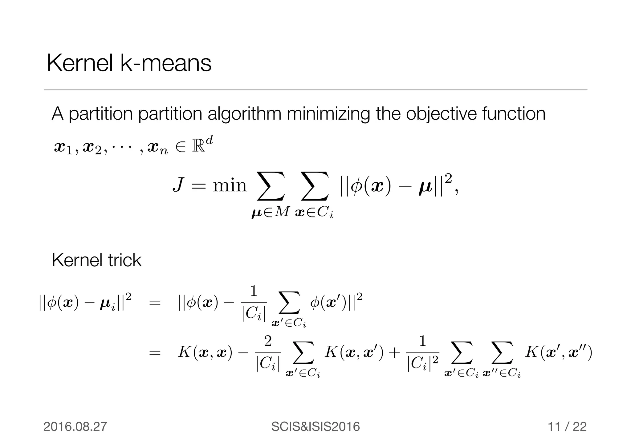
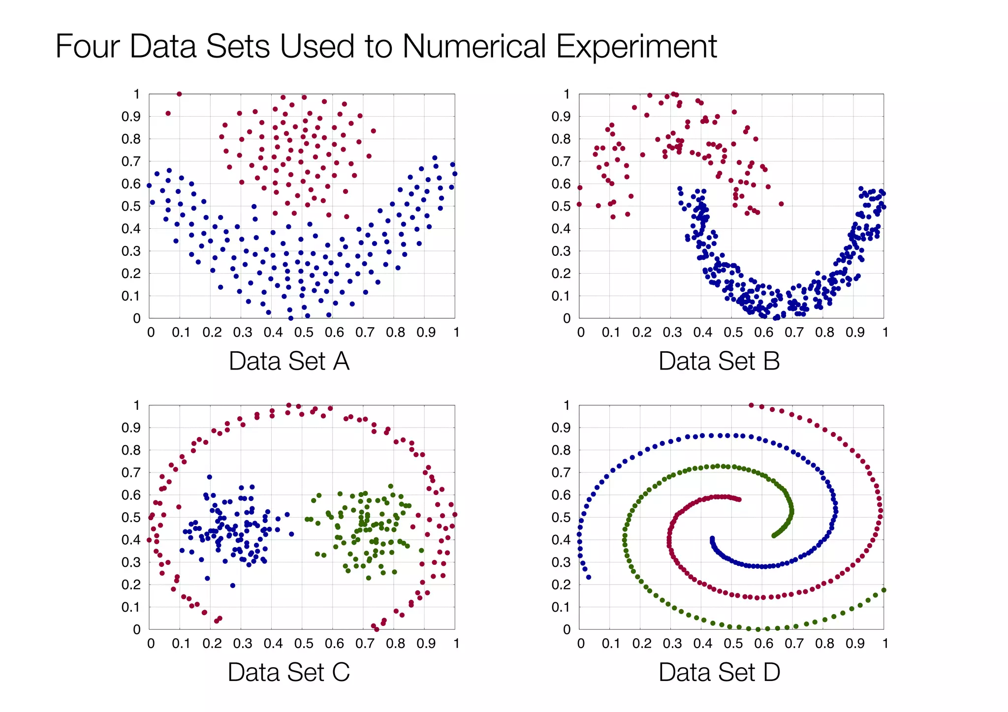
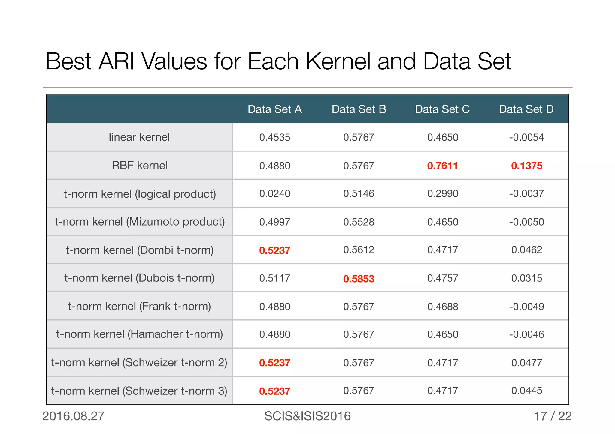
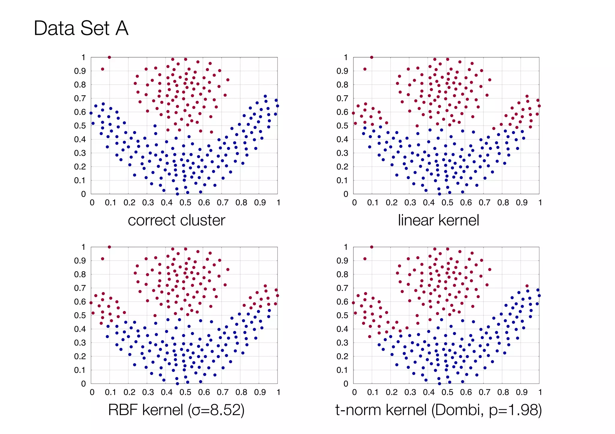
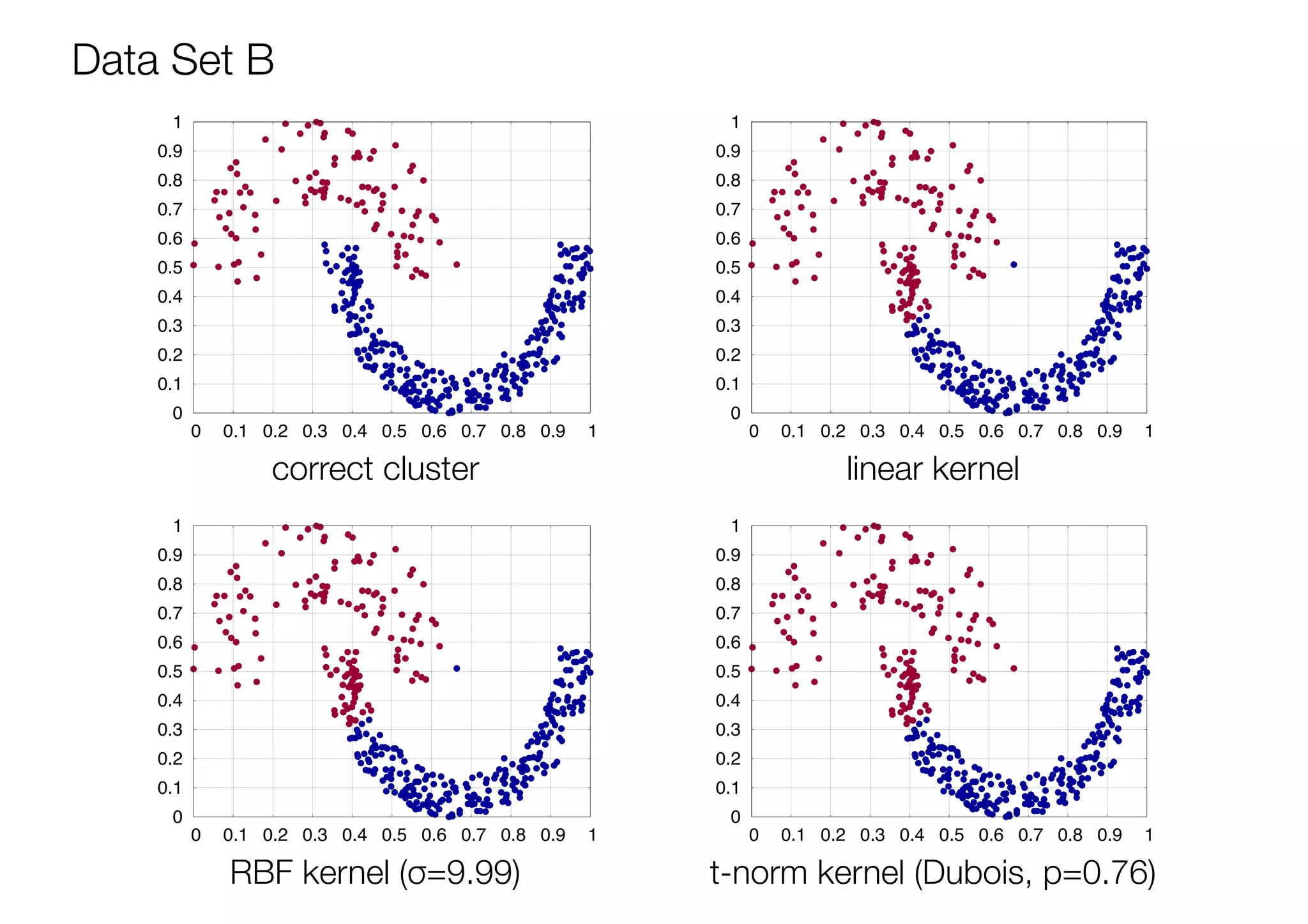
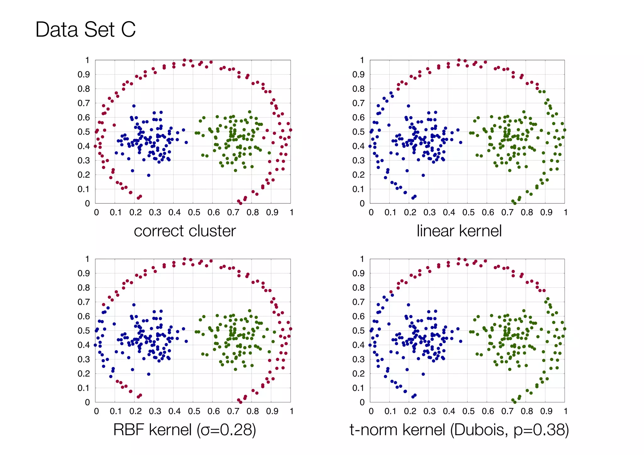
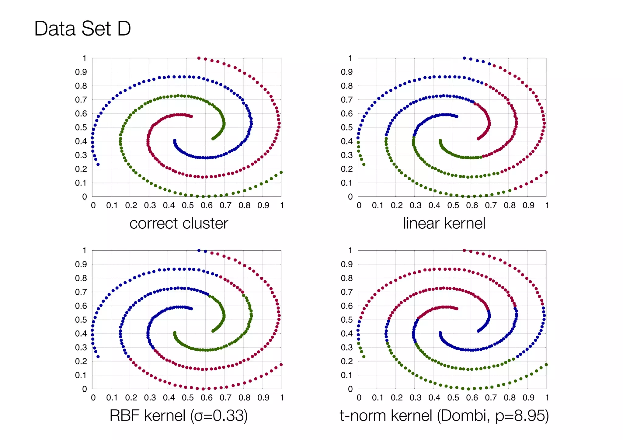
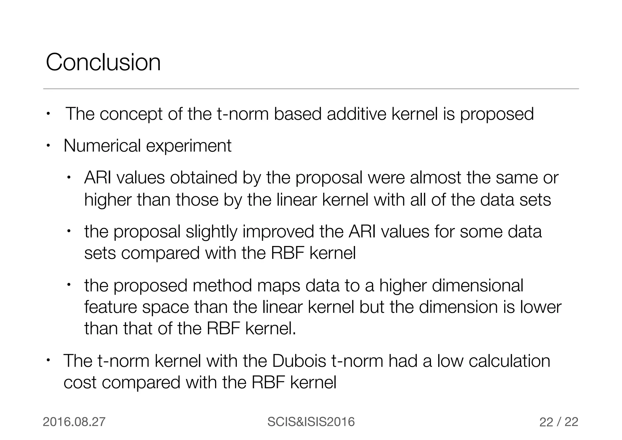
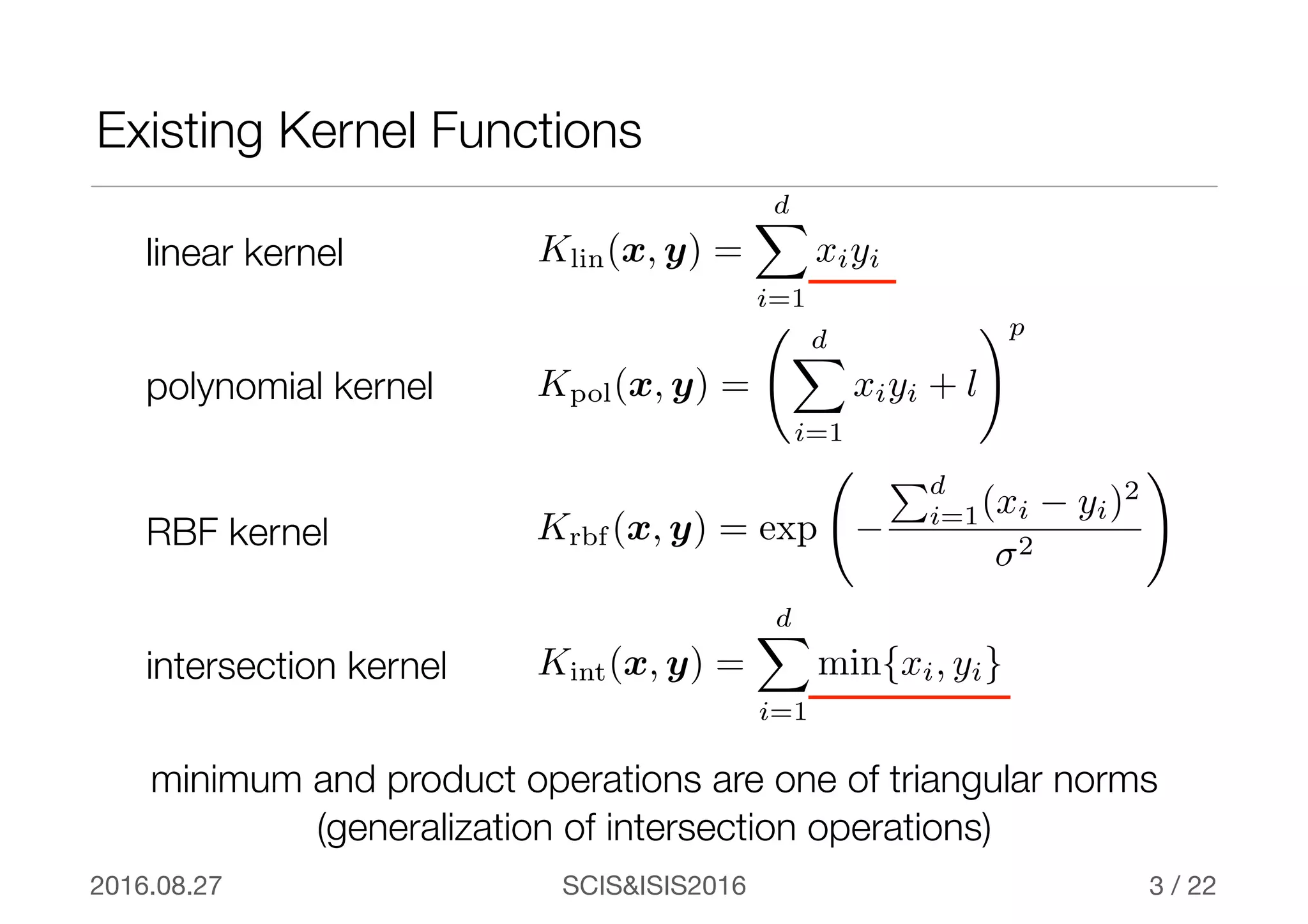
/ 22SCIS&ISIS20162016.08.27
Families of Triangular Norm Based Kernel Function
and Its Application to Kernel k-means
Kazushi Okamoto
The University of Electro-Communications
1
/ 22SCIS&ISIS20162016.08.27
Introduction
• A kernel method is a fundamental and important pattern analysis
approach based on a kernel function
• It is used in machine learning tasks such as classification,
clustering, and dimension reduction
• A kernel function corresponds to a similarity measure between
two data
• mapping each data to a high-dimensional feature space
• inner product on that space
2
SCIS&ISIS20162016.08.27 / 22
Existing Kernel Functions
3
linear kernel Klin(x, y) =
dX
i=1
xiyi
Kpol(x, y) =
dX
i=1
xiyi + l
!p
Krbf (x, y) = exp −
Pd
i=1(xi − yi)2
σ2
!
Kint(x, y) =
dX
i=1
min{xi, yi}
polynomial kernel
RBF kernel
intersection kernel
minimum and product operations are one of triangular norms
(generalization of intersection operations)
SCIS&ISIS20162016.08.27 / 22
A function is a positive semi-definite kernel if and only ifK
Positive Semi-Definite Kernel
4
K : ⌦ ⇥ ⌦ −! R 8x, y 2 ⌦ 8x1, x2, · · · , xm 2 ⌦
K(x, y) = K(y, x)
mX
i=1
mX
j=1
cicjK(xi, xj) ≥ 0 8ci, cj 2 R
1)
2)
Kernel calculation means inner product on the feature space φ
K(x, y) = φ(x) · φ(y)
8m 2 N+
A set is assumed real-valued vector, graph, and string⌦
(quadratic form)
SCIS&ISIS20162016.08.27 / 22
Additive Kernel
5
K : Rd
⇥ Rd
−! R 8x, y 2 Rd
K(x, y) =
dX
i=1
Ki(xi, yi)
Ki : R ⇥ R −! R
8KiIf is positive semi-definite, then the additive kernel
is also positive semi-definite kernel, since
K
mX
j=1
mX
k=1
cjckK(x, y) =
mX
j=1
mX
k=1
cjck
dX
i=1
Ki(xi, yi)
=
dX
i=1
mX
j=1
mX
k=1
cjckKi(xi, yi) ≥ 0
5
SCIS&ISIS20162016.08.27 / 22
Triangular norm (t-norm)
6
A function is called t-norm if and only ifT
T(x, 1) = x
T(x, y) = T(y, x)
T(x, T(y, z)) = T(T(x, y), z)
T(x, y)  T(x, z) y  zif
1)
2)
3)
4)
T : [0, 1] ⇥ [0, 1] −! [0, 1] 8x, y, z 2 [0, 1]
According to fuzzy logic, t-norms represent intersection operations
SCIS&ISIS20162016.08.27 / 22
Example of t-norms
7
Hamacher t-norm
(p = 0.4)
0 0.2 0.4 0.6 0.8 1 0
0.2
0.4
0.6
0.8
1
0
0.2
0.4
0.6
0.8
1
x
y
Dubois t-norm
(p = 0.4)
0 0.2 0.4 0.6 0.8 1 0
0.2
0.4
0.6
0.8
1
0
0.2
0.4
0.6
0.8
1
x
y
Hamacher t-norm
Dubois t-norm Tdb(x, y) =
xy
max {x, y, p}
Th(x, y) =
xy
p + (1 − p)(x + y − xy)
p 2 [0, 1]
p 2 [0, 1]
SCIS&ISIS20162016.08.27 / 22
all principal minors of is
Is t-norm Positive Semi-Definite on [0, 1] ?
8
A =
0
B
B
B
@
T(x1, x1) T(x1, x2) · · · T(x1, xm)
T(x2, x1) T(x2, x2) · · · T(x2, xm)
...
...
...
...
T(xm, x1) T(xm, x2) · · · T(xm, xm)
1
C
C
C
A
Condition of positive semi-definite
A ≥ 0
8ci, cj 2 R 8m 2 N+
()A is positive semi-definite
mX
i=1
mX
j=1
cicjT(xi, xj)
SCIS&ISIS20162016.08.27 / 22
Is t-norm Positive Semi-Definite on [0, 1] ?
9
m = 2
✓
T(x1, x1) T(x1, x2)
T(x2, x1) T(x2, x2)
◆
|T(x1, x1)| ≥ 0
|T(x2, x2)| ≥ 0
T(x1, x1) T(x1, x2)
T(x2, x1) T(x2, x2)
m = 1
1X
i=1
1X
j=1
cicjT(xi, xi) = c2
i T(xi, xi) ≥ 0
all principal minors of are ≥ 0
SCIS&ISIS20162016.08.27 / 22
Is t-norm Positive Semi-Definite on [0, 1] ?
10
T(x1, x1) T(x1, x2)
T(x2, x1) T(x2, x2)
= T(x1, x1)T(x2, x2) − T2
(x1, x2)
T(x, y) ≥ Ta(x, y) = xy8x, y z · T(x, y)  T(x, zy)=)
T(0, x2) = 0 < x1 < x2 = T(1, x2) x1 = T(w, x2)
T(x1, x2)
T(x2, x2)
T(w, T(x2, x2))  T(w, T(x1, x2))
T(x2, x2)
T(x1, x2)
≥
T(w, T(x2, x2))
T(w, T(x1, x2))
=
T(T(w, x2), x2)
T(T(w, x2), x1)
=
T(x1, x2)
T(x1, x1)
SCIS&ISIS20162016.08.27 / 22
Kernel k-means
11
A partition partition algorithm minimizing the objective function
J = min
X
µ2M
X
x2Ci
||φ(x) − µ||2
,
x1, x2, · · · , xn 2 Rd
||φ(x) − µi||2
= ||φ(x) −
1
|Ci|
X
x02Ci
φ(x0
)||2
= K(x, x) −
2
|Ci|
X
x02Ci
K(x, x0
) +
1
|Ci|2
X
x02Ci
X
x002Ci
K(x0
, x00
)
Kernel trick
/ 22SCIS&ISIS20162016.08.27
Conditions of Clustering Experiment
• each clustering process was terminated when the number of
iterations reached 1,000, or the difference between the latest
and current objective function values was less than 10-4
• one partition that minimized the objective function was
determined within 100 attempts using different initial partitions
• number of clusters was determined depending on the data set
12
SCIS&ISIS20162016.08.27 / 22
Applied Kernel Functions
13
linear kernel Klin(x, y) =
dX
i=1
xiyi
Krbf (x, y) = exp −
Pd
i=1(xi − yi)2
σ2
!
RBF kernel
Kt(x, y) =
dX
i=1
Ti(xi, yi)t-norm kernel
Applied non-parameterized t-norms
Tmp(x, y) =
2
⇡
cot−1
✓
cot
1
2
⇡x + cot
1
2
⇡y
◆
Mizumoto product
Tl(x, y) = min{x, y}logical product
SCIS&ISIS20162016.08.27 / 22
Applied Parameterized t-norms
14
Tdm(x, y) =
1
1 + p
r
�1−x
x
�p
+
⇣
1−y
y
⌘p
Tdb(x, y) =
xy
max {x, y, p}
Dubois t-norm
Dombi t-norm
Tf (x, y) = logp
✓
1 +
(px
− 1)(py
− 1)
p − 1
◆
Frank t-norm
Th(x, y) =
xy
p + (1 − p)(x + y − xy)
Hamacher t-norm
Ts2(x, y) =
1
p
q
1
xp + 1
yp − 1
Ts3(x, y) = 1 − p
p
(1 − x)p + (1 − y)p − (1 − x)p(1 − y)p
Schweizer t-norm 2
Schweizer t-norm 3
SCIS&ISIS20162016.08.27 / 22
Evaluation Measure: Adjusted Rand Index (ARI)
15
ARI =
MX
i=1
NX
j=1
nij C2 −
ab
nC2
1
2
(a + b) −
ab
nC2
a =
MX
i=1
ni· C2
b =
NX
j=1
n·j C2
U = {u1, u2, · · · , uM } V = {v1, v2, · · · , vN }
nij = |ui  vj|
ni· =
NX
j=1
nijn·j =
MX
i=1
nij n =
MX
i=1
NX
j=1
nij
0
0.1
0.2
0.3
0.4
0.5
0.6
0.7
0.8
0.9
1
0 0.1 0.2 0.3 0.4 0.5 0.6 0.7 0.8 0.9 1
0
0.1
0.2
0.3
0.4
0.5
0.6
0.7
0.8
0.9
1
0 0.1 0.2 0.3 0.4 0.5 0.6 0.7 0.8 0.9 1
0
0.1
0.2
0.3
0.4
0.5
0.6
0.7
0.8
0.9
1
0 0.1 0.2 0.3 0.4 0.5 0.6 0.7 0.8 0.9 1
0
0.1
0.2
0.3
0.4
0.5
0.6
0.7
0.8
0.9
1
0 0.1 0.2 0.3 0.4 0.5 0.6 0.7 0.8 0.9 1
Four Data Sets Used to Numerical Experiment
Data Set BData Set A
Data Set C Data Set D
SCIS&ISIS20162016.08.27 / 22
Best ARI Values for Each Kernel and Data Set
17
Data Set A Data Set B Data Set C Data Set D
linear kernel 0.4535 0.5767 0.4650 -0.0054
RBF kernel 0.4880 0.5767 0.7611 0.1375
t-norm kernel (logical product) 0.0240 0.5146 0.2990 -0.0037
t-norm kernel (Mizumoto product) 0.4997 0.5528 0.4650 -0.0050
t-norm kernel (Dombi t-norm) 0.5237 0.5612 0.4717 0.0462
t-norm kernel (Dubois t-norm) 0.5117 0.5853 0.4757 0.0315
t-norm kernel (Frank t-norm) 0.4880 0.5767 0.4688 -0.0049
t-norm kernel (Hamacher t-norm) 0.4880 0.5767 0.4650 -0.0046
t-norm kernel (Schweizer t-norm 2) 0.5237 0.5767 0.4717 0.0477
t-norm kernel (Schweizer t-norm 3) 0.5237 0.5767 0.4717 0.0445
0
0.1
0.2
0.3
0.4
0.5
0.6
0.7
0.8
0.9
1
0 0.1 0.2 0.3 0.4 0.5 0.6 0.7 0.8 0.9 1
0
0.1
0.2
0.3
0.4
0.5
0.6
0.7
0.8
0.9
1
0 0.1 0.2 0.3 0.4 0.5 0.6 0.7 0.8 0.9 1
0
0.1
0.2
0.3
0.4
0.5
0.6
0.7
0.8
0.9
1
0 0.1 0.2 0.3 0.4 0.5 0.6 0.7 0.8 0.9 1
0
0.1
0.2
0.3
0.4
0.5
0.6
0.7
0.8
0.9
1
0 0.1 0.2 0.3 0.4 0.5 0.6 0.7 0.8 0.9 1
Data Set A
linear kernel
RBF kernel (σ=8.52)
correct cluster
t-norm kernel (Dombi, p=1.98)
0
0.1
0.2
0.3
0.4
0.5
0.6
0.7
0.8
0.9
1
0 0.1 0.2 0.3 0.4 0.5 0.6 0.7 0.8 0.9 1
0
0.1
0.2
0.3
0.4
0.5
0.6
0.7
0.8
0.9
1
0 0.1 0.2 0.3 0.4 0.5 0.6 0.7 0.8 0.9 1
0
0.1
0.2
0.3
0.4
0.5
0.6
0.7
0.8
0.9
1
0 0.1 0.2 0.3 0.4 0.5 0.6 0.7 0.8 0.9 1
Data Set B
linear kernel
RBF kernel (σ=9.99)
correct cluster
t-norm kernel (Dubois, p=0.76)
0
0.1
0.2
0.3
0.4
0.5
0.6
0.7
0.8
0.9
1
0 0.1 0.2 0.3 0.4 0.5 0.6 0.7 0.8 0.9 1
0
0.1
0.2
0.3
0.4
0.5
0.6
0.7
0.8
0.9
1
0 0.1 0.2 0.3 0.4 0.5 0.6 0.7 0.8 0.9 1
0
0.1
0.2
0.3
0.4
0.5
0.6
0.7
0.8
0.9
1
0 0.1 0.2 0.3 0.4 0.5 0.6 0.7 0.8 0.9 1
0
0.1
0.2
0.3
0.4
0.5
0.6
0.7
0.8
0.9
1
0 0.1 0.2 0.3 0.4 0.5 0.6 0.7 0.8 0.9 1
0
0.1
0.2
0.3
0.4
0.5
0.6
0.7
0.8
0.9
1
0 0.1 0.2 0.3 0.4 0.5 0.6 0.7 0.8 0.9 1
Data Set C
linear kernel
RBF kernel (σ=0.28)
correct cluster
t-norm kernel (Dubois, p=0.38)
0
0.1
0.2
0.3
0.4
0.5
0.6
0.7
0.8
0.9
1
0 0.1 0.2 0.3 0.4 0.5 0.6 0.7 0.8 0.9 1
0
0.1
0.2
0.3
0.4
0.5
0.6
0.7
0.8
0.9
1
0 0.1 0.2 0.3 0.4 0.5 0.6 0.7 0.8 0.9 1
0
0.1
0.2
0.3
0.4
0.5
0.6
0.7
0.8
0.9
1
0 0.1 0.2 0.3 0.4 0.5 0.6 0.7 0.8 0.9 1
0
0.1
0.2
0.3
0.4
0.5
0.6
0.7
0.8
0.9
1
0 0.1 0.2 0.3 0.4 0.5 0.6 0.7 0.8 0.9 1
Data Set D
linear kernel
RBF kernel (σ=0.33)
correct cluster
t-norm kernel (Dombi, p=8.95)
/ 22SCIS&ISIS20162016.08.27
Conclusion
• The concept of the t-norm based additive kernel is proposed
• Numerical experiment
• ARI values obtained by the proposal were almost the same or
higher than those by the linear kernel with all of the data sets
• the proposal slightly improved the ARI values for some data
sets compared with the RBF kernel
• the proposed method maps data to a higher dimensional
feature space than the linear kernel but the dimension is lower
than that of the RBF kernel.
• The t-norm kernel with the Dubois t-norm had a low calculation
cost compared with the RBF kernel
22

Families of Triangular Norm Based Kernel Function and Its Application to Kernel k-means

  • 1.
    / 22SCIS&ISIS20162016.08.27 Families ofTriangular Norm Based Kernel Function and Its Application to Kernel k-means Kazushi Okamoto The University of Electro-Communications 1
  • 2.
    / 22SCIS&ISIS20162016.08.27 Introduction • Akernel method is a fundamental and important pattern analysis approach based on a kernel function • It is used in machine learning tasks such as classification, clustering, and dimension reduction • A kernel function corresponds to a similarity measure between two data • mapping each data to a high-dimensional feature space • inner product on that space 2
  • 3.
    SCIS&ISIS20162016.08.27 / 22 ExistingKernel Functions 3 linear kernel Klin(x, y) = dX i=1 xiyi Kpol(x, y) = dX i=1 xiyi + l !p Krbf (x, y) = exp − Pd i=1(xi − yi)2 σ2 ! Kint(x, y) = dX i=1 min{xi, yi} polynomial kernel RBF kernel intersection kernel minimum and product operations are one of triangular norms (generalization of intersection operations)
  • 4.
    SCIS&ISIS20162016.08.27 / 22 Afunction is a positive semi-definite kernel if and only ifK Positive Semi-Definite Kernel 4 K : ⌦ ⇥ ⌦ −! R 8x, y 2 ⌦ 8x1, x2, · · · , xm 2 ⌦ K(x, y) = K(y, x) mX i=1 mX j=1 cicjK(xi, xj) ≥ 0 8ci, cj 2 R 1) 2) Kernel calculation means inner product on the feature space φ K(x, y) = φ(x) · φ(y) 8m 2 N+ A set is assumed real-valued vector, graph, and string⌦ (quadratic form)
  • 5.
    SCIS&ISIS20162016.08.27 / 22 AdditiveKernel 5 K : Rd ⇥ Rd −! R 8x, y 2 Rd K(x, y) = dX i=1 Ki(xi, yi) Ki : R ⇥ R −! R 8KiIf is positive semi-definite, then the additive kernel is also positive semi-definite kernel, since K mX j=1 mX k=1 cjckK(x, y) = mX j=1 mX k=1 cjck dX i=1 Ki(xi, yi) = dX i=1 mX j=1 mX k=1 cjckKi(xi, yi) ≥ 0 5
  • 6.
    SCIS&ISIS20162016.08.27 / 22 Triangularnorm (t-norm) 6 A function is called t-norm if and only ifT T(x, 1) = x T(x, y) = T(y, x) T(x, T(y, z)) = T(T(x, y), z) T(x, y)  T(x, z) y  zif 1) 2) 3) 4) T : [0, 1] ⇥ [0, 1] −! [0, 1] 8x, y, z 2 [0, 1] According to fuzzy logic, t-norms represent intersection operations
  • 7.
    SCIS&ISIS20162016.08.27 / 22 Exampleof t-norms 7 Hamacher t-norm (p = 0.4) 0 0.2 0.4 0.6 0.8 1 0 0.2 0.4 0.6 0.8 1 0 0.2 0.4 0.6 0.8 1 x y Dubois t-norm (p = 0.4) 0 0.2 0.4 0.6 0.8 1 0 0.2 0.4 0.6 0.8 1 0 0.2 0.4 0.6 0.8 1 x y Hamacher t-norm Dubois t-norm Tdb(x, y) = xy max {x, y, p} Th(x, y) = xy p + (1 − p)(x + y − xy) p 2 [0, 1] p 2 [0, 1]
  • 8.
    SCIS&ISIS20162016.08.27 / 22 allprincipal minors of is Is t-norm Positive Semi-Definite on [0, 1] ? 8 A = 0 B B B @ T(x1, x1) T(x1, x2) · · · T(x1, xm) T(x2, x1) T(x2, x2) · · · T(x2, xm) ... ... ... ... T(xm, x1) T(xm, x2) · · · T(xm, xm) 1 C C C A Condition of positive semi-definite A ≥ 0 8ci, cj 2 R 8m 2 N+ ()A is positive semi-definite mX i=1 mX j=1 cicjT(xi, xj)
  • 9.
    SCIS&ISIS20162016.08.27 / 22 Ist-norm Positive Semi-Definite on [0, 1] ? 9 m = 2 ✓ T(x1, x1) T(x1, x2) T(x2, x1) T(x2, x2) ◆ |T(x1, x1)| ≥ 0 |T(x2, x2)| ≥ 0 T(x1, x1) T(x1, x2) T(x2, x1) T(x2, x2) m = 1 1X i=1 1X j=1 cicjT(xi, xi) = c2 i T(xi, xi) ≥ 0 all principal minors of are ≥ 0
  • 10.
    SCIS&ISIS20162016.08.27 / 22 Ist-norm Positive Semi-Definite on [0, 1] ? 10 T(x1, x1) T(x1, x2) T(x2, x1) T(x2, x2) = T(x1, x1)T(x2, x2) − T2 (x1, x2) T(x, y) ≥ Ta(x, y) = xy8x, y z · T(x, y)  T(x, zy)=) T(0, x2) = 0 < x1 < x2 = T(1, x2) x1 = T(w, x2) T(x1, x2) T(x2, x2) T(w, T(x2, x2))  T(w, T(x1, x2)) T(x2, x2) T(x1, x2) ≥ T(w, T(x2, x2)) T(w, T(x1, x2)) = T(T(w, x2), x2) T(T(w, x2), x1) = T(x1, x2) T(x1, x1)
  • 11.
    SCIS&ISIS20162016.08.27 / 22 Kernelk-means 11 A partition partition algorithm minimizing the objective function J = min X µ2M X x2Ci ||φ(x) − µ||2 , x1, x2, · · · , xn 2 Rd ||φ(x) − µi||2 = ||φ(x) − 1 |Ci| X x02Ci φ(x0 )||2 = K(x, x) − 2 |Ci| X x02Ci K(x, x0 ) + 1 |Ci|2 X x02Ci X x002Ci K(x0 , x00 ) Kernel trick
  • 12.
    / 22SCIS&ISIS20162016.08.27 Conditions ofClustering Experiment • each clustering process was terminated when the number of iterations reached 1,000, or the difference between the latest and current objective function values was less than 10-4 • one partition that minimized the objective function was determined within 100 attempts using different initial partitions • number of clusters was determined depending on the data set 12
  • 13.
    SCIS&ISIS20162016.08.27 / 22 AppliedKernel Functions 13 linear kernel Klin(x, y) = dX i=1 xiyi Krbf (x, y) = exp − Pd i=1(xi − yi)2 σ2 ! RBF kernel Kt(x, y) = dX i=1 Ti(xi, yi)t-norm kernel Applied non-parameterized t-norms Tmp(x, y) = 2 ⇡ cot−1 ✓ cot 1 2 ⇡x + cot 1 2 ⇡y ◆ Mizumoto product Tl(x, y) = min{x, y}logical product
  • 14.
    SCIS&ISIS20162016.08.27 / 22 AppliedParameterized t-norms 14 Tdm(x, y) = 1 1 + p r �1−x x �p + ⇣ 1−y y ⌘p Tdb(x, y) = xy max {x, y, p} Dubois t-norm Dombi t-norm Tf (x, y) = logp ✓ 1 + (px − 1)(py − 1) p − 1 ◆ Frank t-norm Th(x, y) = xy p + (1 − p)(x + y − xy) Hamacher t-norm Ts2(x, y) = 1 p q 1 xp + 1 yp − 1 Ts3(x, y) = 1 − p p (1 − x)p + (1 − y)p − (1 − x)p(1 − y)p Schweizer t-norm 2 Schweizer t-norm 3
  • 15.
    SCIS&ISIS20162016.08.27 / 22 EvaluationMeasure: Adjusted Rand Index (ARI) 15 ARI = MX i=1 NX j=1 nij C2 − ab nC2 1 2 (a + b) − ab nC2 a = MX i=1 ni· C2 b = NX j=1 n·j C2 U = {u1, u2, · · · , uM } V = {v1, v2, · · · , vN } nij = |ui vj| ni· = NX j=1 nijn·j = MX i=1 nij n = MX i=1 NX j=1 nij
  • 16.
    0 0.1 0.2 0.3 0.4 0.5 0.6 0.7 0.8 0.9 1 0 0.1 0.20.3 0.4 0.5 0.6 0.7 0.8 0.9 1 0 0.1 0.2 0.3 0.4 0.5 0.6 0.7 0.8 0.9 1 0 0.1 0.2 0.3 0.4 0.5 0.6 0.7 0.8 0.9 1 0 0.1 0.2 0.3 0.4 0.5 0.6 0.7 0.8 0.9 1 0 0.1 0.2 0.3 0.4 0.5 0.6 0.7 0.8 0.9 1 0 0.1 0.2 0.3 0.4 0.5 0.6 0.7 0.8 0.9 1 0 0.1 0.2 0.3 0.4 0.5 0.6 0.7 0.8 0.9 1 Four Data Sets Used to Numerical Experiment Data Set BData Set A Data Set C Data Set D
  • 17.
    SCIS&ISIS20162016.08.27 / 22 BestARI Values for Each Kernel and Data Set 17 Data Set A Data Set B Data Set C Data Set D linear kernel 0.4535 0.5767 0.4650 -0.0054 RBF kernel 0.4880 0.5767 0.7611 0.1375 t-norm kernel (logical product) 0.0240 0.5146 0.2990 -0.0037 t-norm kernel (Mizumoto product) 0.4997 0.5528 0.4650 -0.0050 t-norm kernel (Dombi t-norm) 0.5237 0.5612 0.4717 0.0462 t-norm kernel (Dubois t-norm) 0.5117 0.5853 0.4757 0.0315 t-norm kernel (Frank t-norm) 0.4880 0.5767 0.4688 -0.0049 t-norm kernel (Hamacher t-norm) 0.4880 0.5767 0.4650 -0.0046 t-norm kernel (Schweizer t-norm 2) 0.5237 0.5767 0.4717 0.0477 t-norm kernel (Schweizer t-norm 3) 0.5237 0.5767 0.4717 0.0445
  • 18.
    0 0.1 0.2 0.3 0.4 0.5 0.6 0.7 0.8 0.9 1 0 0.1 0.20.3 0.4 0.5 0.6 0.7 0.8 0.9 1 0 0.1 0.2 0.3 0.4 0.5 0.6 0.7 0.8 0.9 1 0 0.1 0.2 0.3 0.4 0.5 0.6 0.7 0.8 0.9 1 0 0.1 0.2 0.3 0.4 0.5 0.6 0.7 0.8 0.9 1 0 0.1 0.2 0.3 0.4 0.5 0.6 0.7 0.8 0.9 1 0 0.1 0.2 0.3 0.4 0.5 0.6 0.7 0.8 0.9 1 0 0.1 0.2 0.3 0.4 0.5 0.6 0.7 0.8 0.9 1 Data Set A linear kernel RBF kernel (σ=8.52) correct cluster t-norm kernel (Dombi, p=1.98)
  • 19.
    0 0.1 0.2 0.3 0.4 0.5 0.6 0.7 0.8 0.9 1 0 0.1 0.20.3 0.4 0.5 0.6 0.7 0.8 0.9 1 0 0.1 0.2 0.3 0.4 0.5 0.6 0.7 0.8 0.9 1 0 0.1 0.2 0.3 0.4 0.5 0.6 0.7 0.8 0.9 1 0 0.1 0.2 0.3 0.4 0.5 0.6 0.7 0.8 0.9 1 0 0.1 0.2 0.3 0.4 0.5 0.6 0.7 0.8 0.9 1 Data Set B linear kernel RBF kernel (σ=9.99) correct cluster t-norm kernel (Dubois, p=0.76) 0 0.1 0.2 0.3 0.4 0.5 0.6 0.7 0.8 0.9 1 0 0.1 0.2 0.3 0.4 0.5 0.6 0.7 0.8 0.9 1
  • 20.
    0 0.1 0.2 0.3 0.4 0.5 0.6 0.7 0.8 0.9 1 0 0.1 0.20.3 0.4 0.5 0.6 0.7 0.8 0.9 1 0 0.1 0.2 0.3 0.4 0.5 0.6 0.7 0.8 0.9 1 0 0.1 0.2 0.3 0.4 0.5 0.6 0.7 0.8 0.9 1 0 0.1 0.2 0.3 0.4 0.5 0.6 0.7 0.8 0.9 1 0 0.1 0.2 0.3 0.4 0.5 0.6 0.7 0.8 0.9 1 0 0.1 0.2 0.3 0.4 0.5 0.6 0.7 0.8 0.9 1 0 0.1 0.2 0.3 0.4 0.5 0.6 0.7 0.8 0.9 1 Data Set C linear kernel RBF kernel (σ=0.28) correct cluster t-norm kernel (Dubois, p=0.38)
  • 21.
    0 0.1 0.2 0.3 0.4 0.5 0.6 0.7 0.8 0.9 1 0 0.1 0.20.3 0.4 0.5 0.6 0.7 0.8 0.9 1 0 0.1 0.2 0.3 0.4 0.5 0.6 0.7 0.8 0.9 1 0 0.1 0.2 0.3 0.4 0.5 0.6 0.7 0.8 0.9 1 0 0.1 0.2 0.3 0.4 0.5 0.6 0.7 0.8 0.9 1 0 0.1 0.2 0.3 0.4 0.5 0.6 0.7 0.8 0.9 1 0 0.1 0.2 0.3 0.4 0.5 0.6 0.7 0.8 0.9 1 0 0.1 0.2 0.3 0.4 0.5 0.6 0.7 0.8 0.9 1 Data Set D linear kernel RBF kernel (σ=0.33) correct cluster t-norm kernel (Dombi, p=8.95)
  • 22.
    / 22SCIS&ISIS20162016.08.27 Conclusion • Theconcept of the t-norm based additive kernel is proposed • Numerical experiment • ARI values obtained by the proposal were almost the same or higher than those by the linear kernel with all of the data sets • the proposal slightly improved the ARI values for some data sets compared with the RBF kernel • the proposed method maps data to a higher dimensional feature space than the linear kernel but the dimension is lower than that of the RBF kernel. • The t-norm kernel with the Dubois t-norm had a low calculation cost compared with the RBF kernel 22