Downloaded 201 times

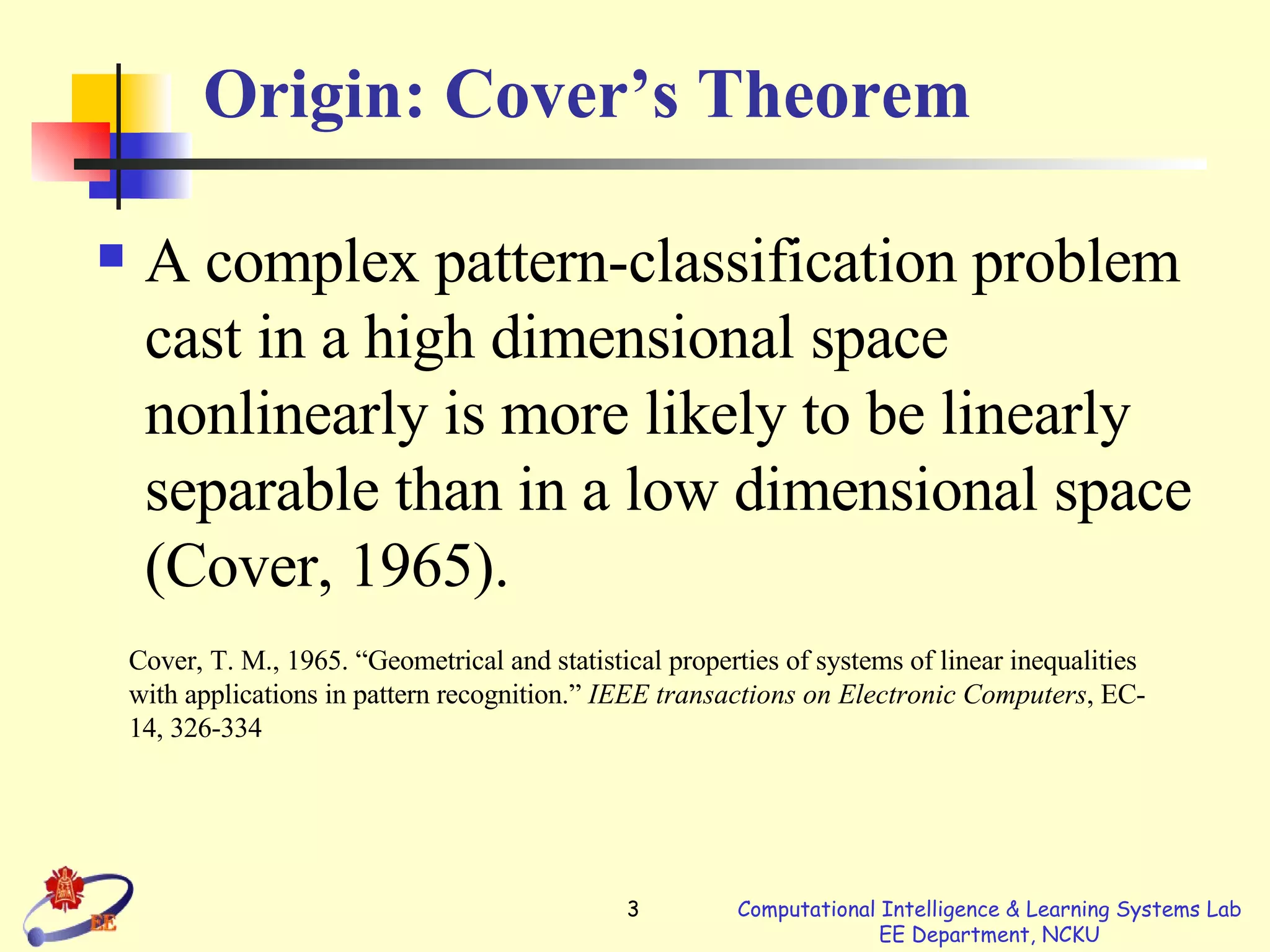
![Cover’s Theorem Covers’ theorem on separability of patterns (1965) x 1 , x 2 , …, x N , x i p , are assigned to two classes C 1 and C 2 -separability: where ( x ) = [ 1 ( x ), 2 ( x ), …, M ( x )] T.](https://image.slidesharecdn.com/section5-rbf-1200980966354718-5/75/Section5-Rbf-4-2048.jpg)


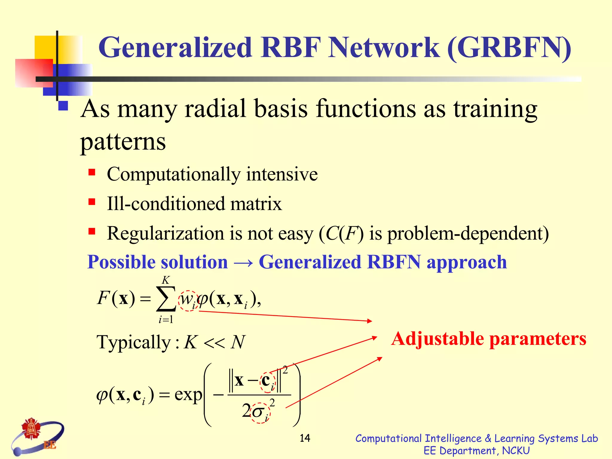

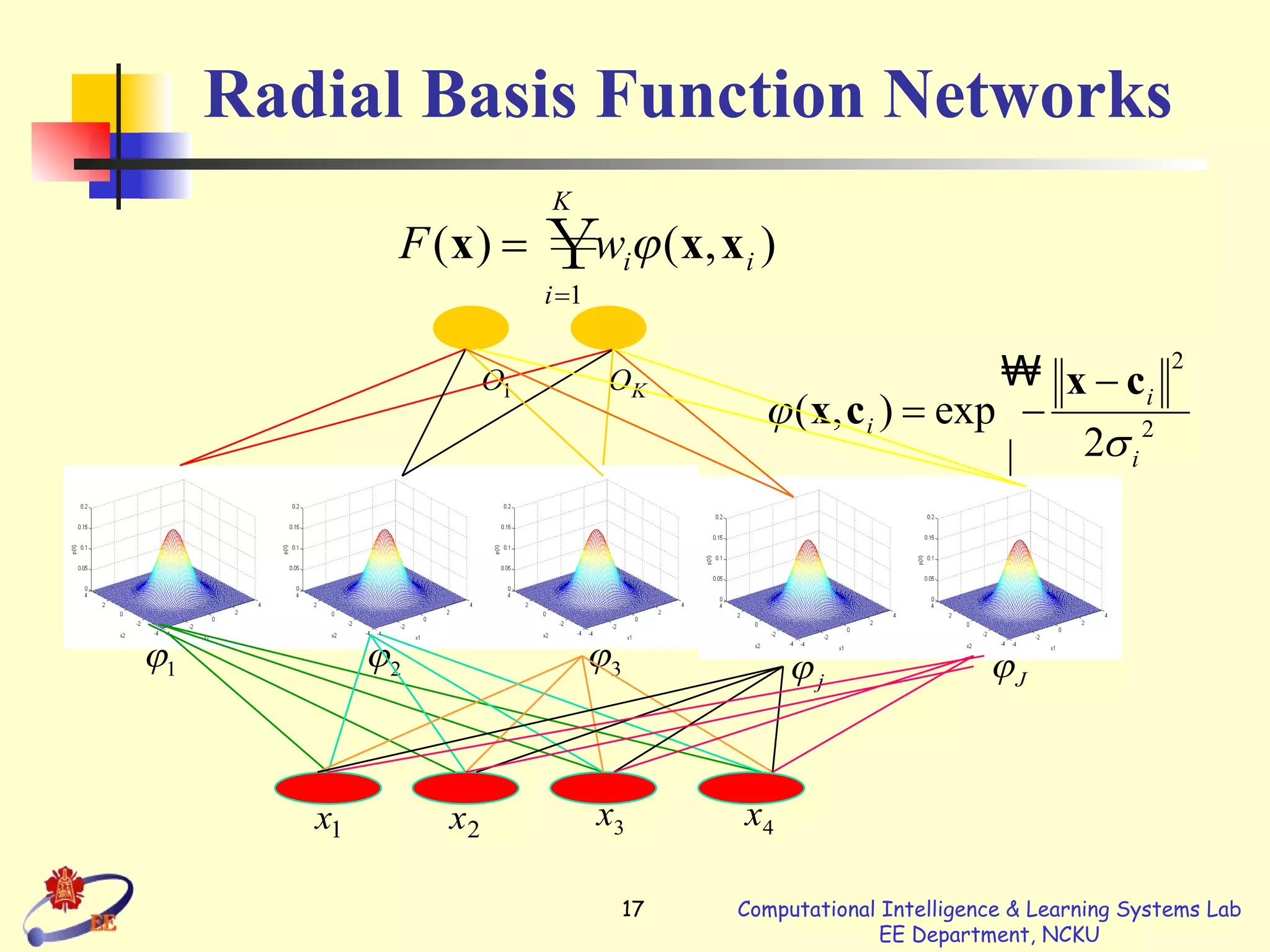


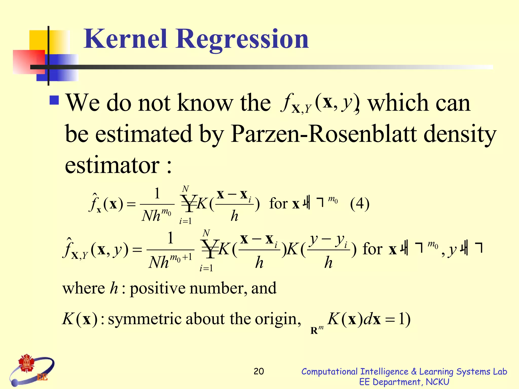


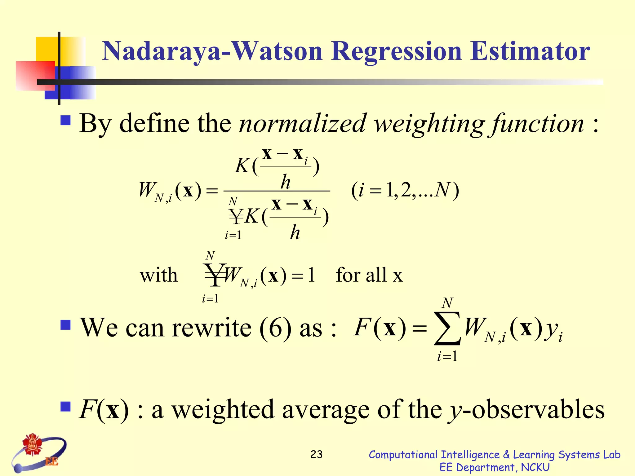

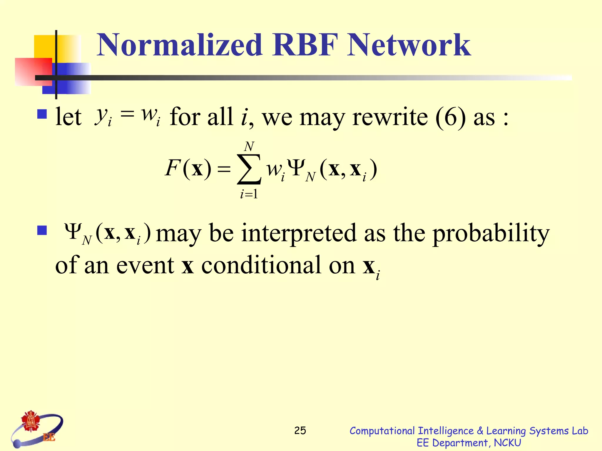


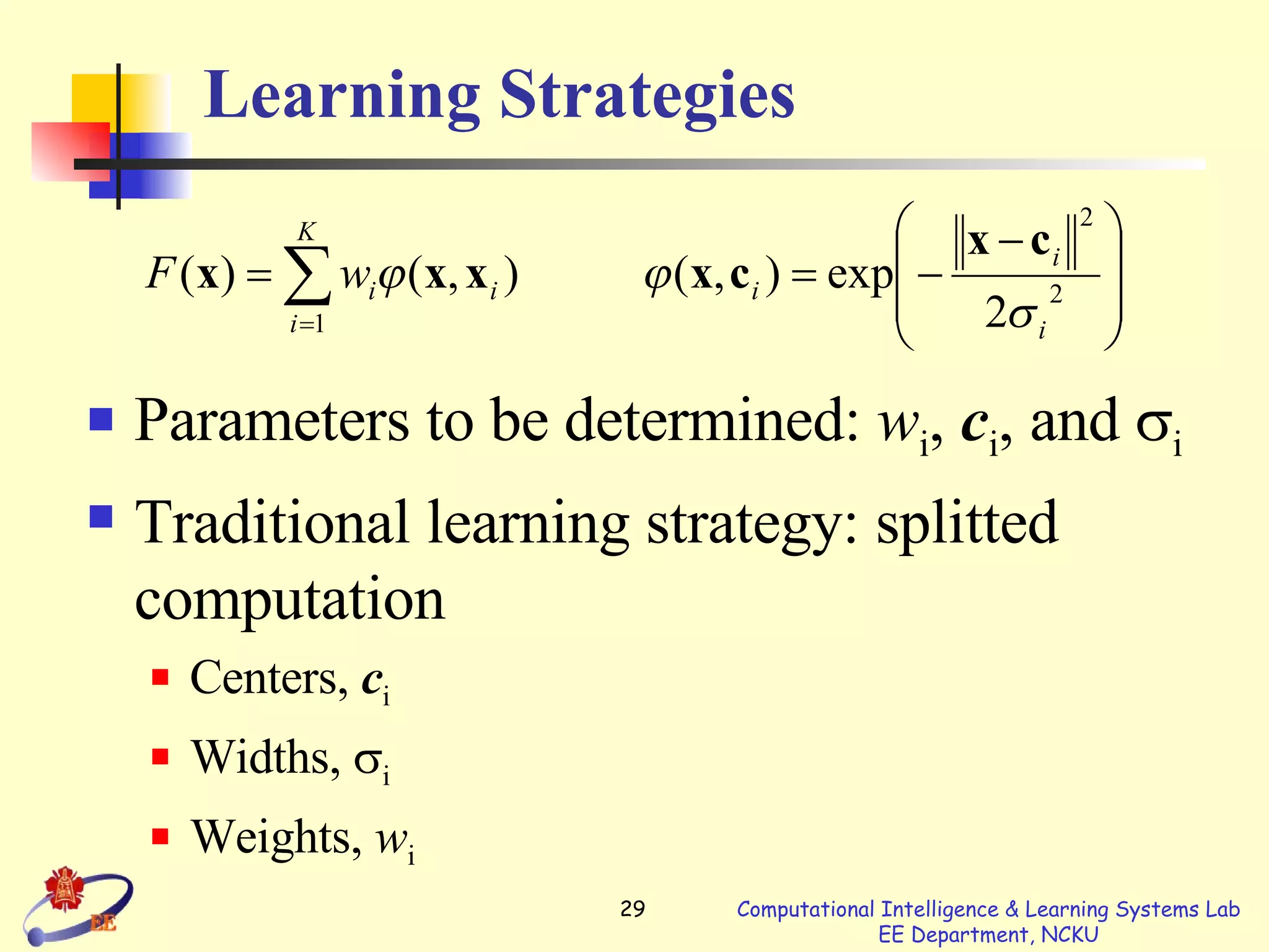


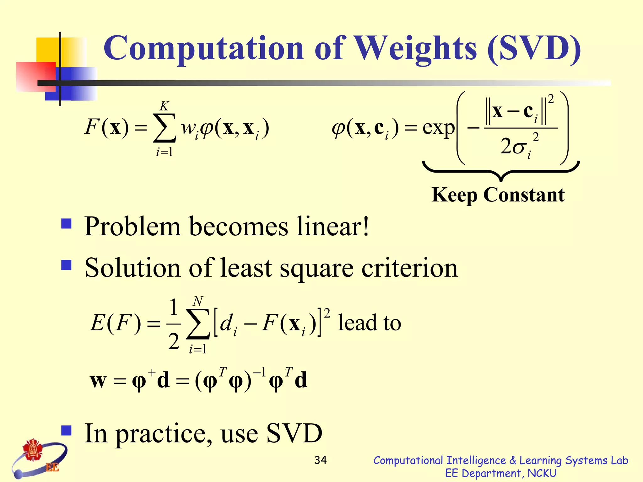
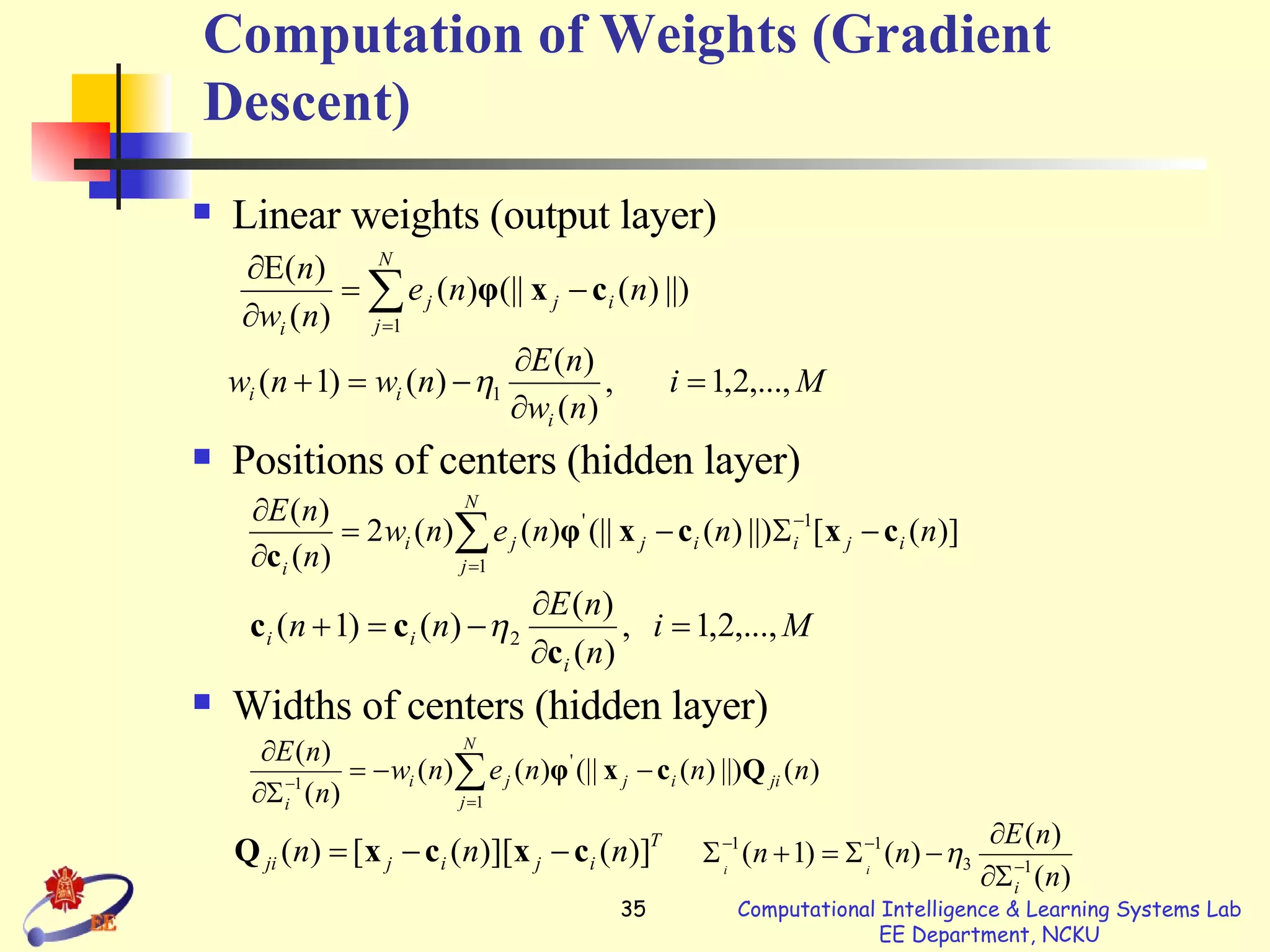
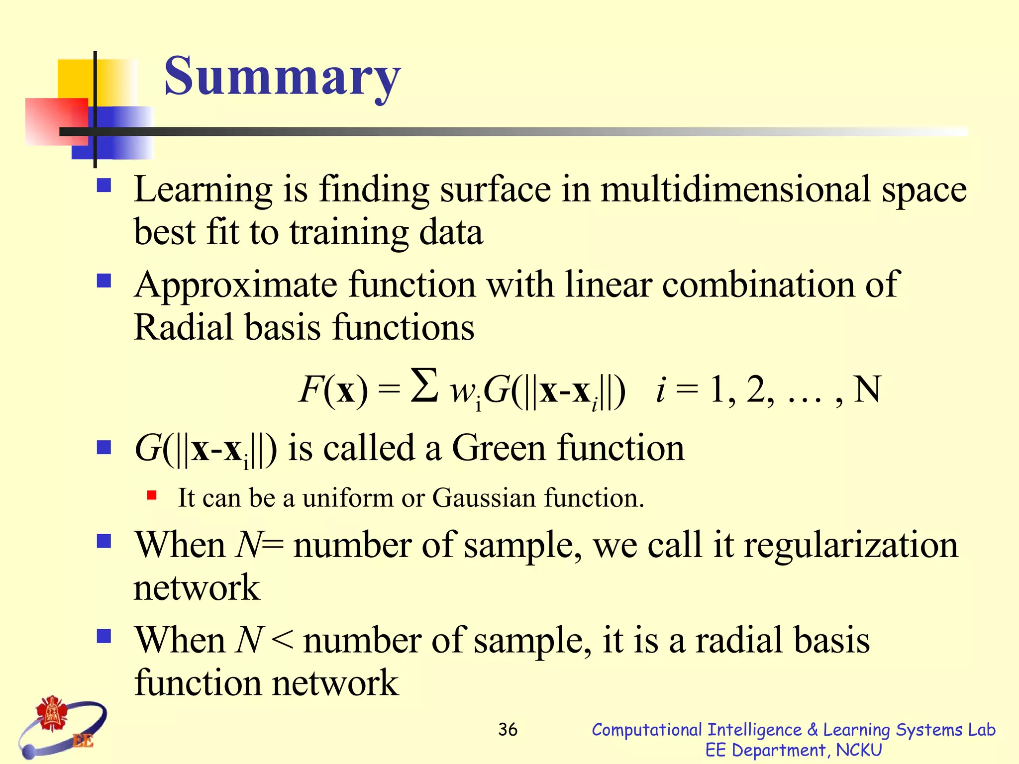

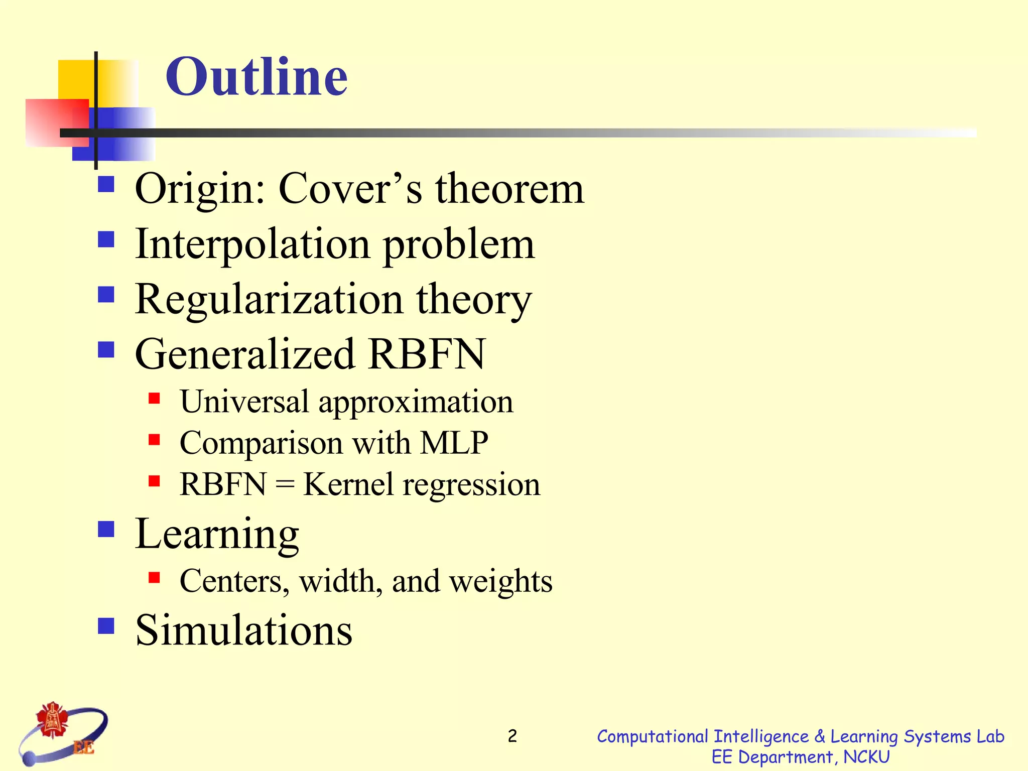
The document summarizes radial basis function (RBF) networks. Key points: - RBF networks use radial basis functions as activation functions and can universally approximate continuous functions. - They are local approximators compared to multilayer perceptrons which are global approximators. - Learning involves determining the centers, widths, and weights. Centers can be randomly selected or via clustering. Widths are usually different for each basis function. Weights are typically learned via least squares or gradient descent methods.