Download as PPS, PPTX
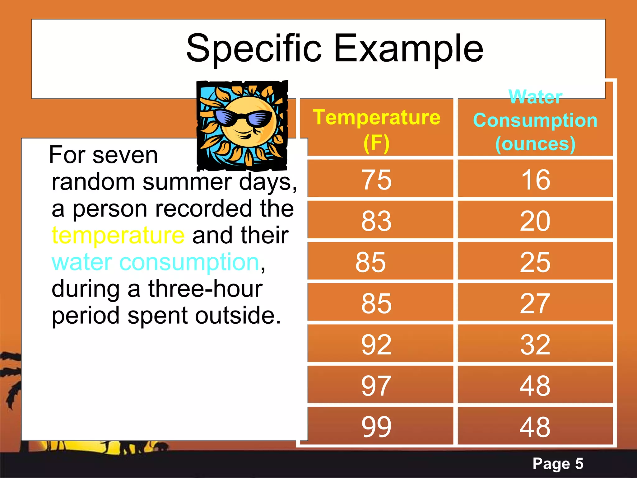
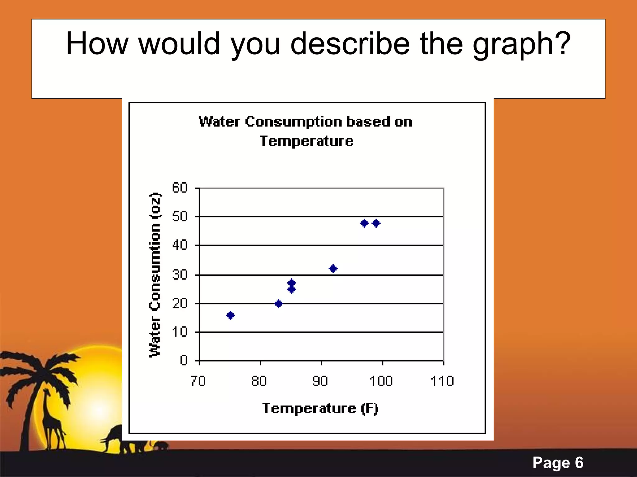
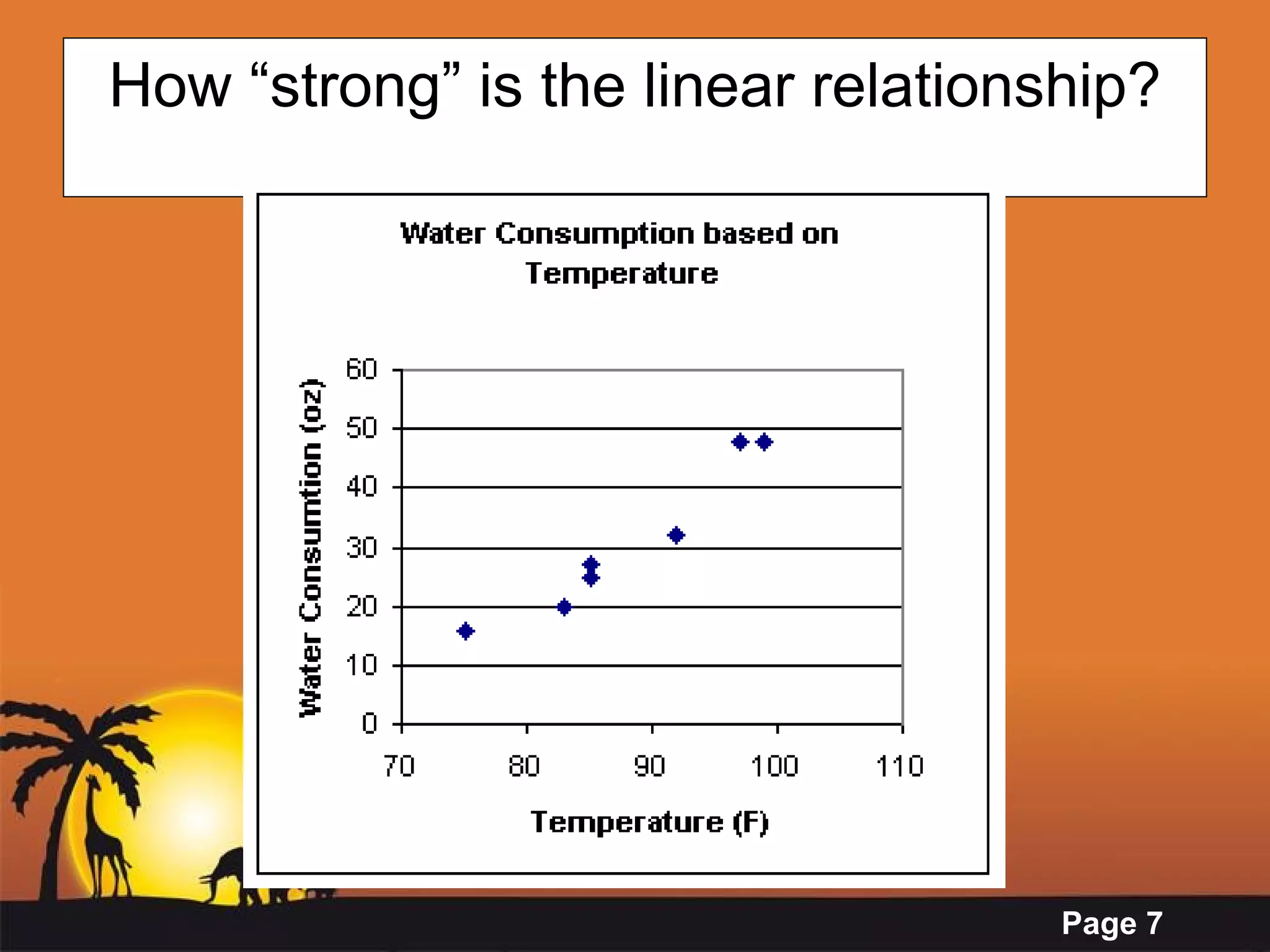
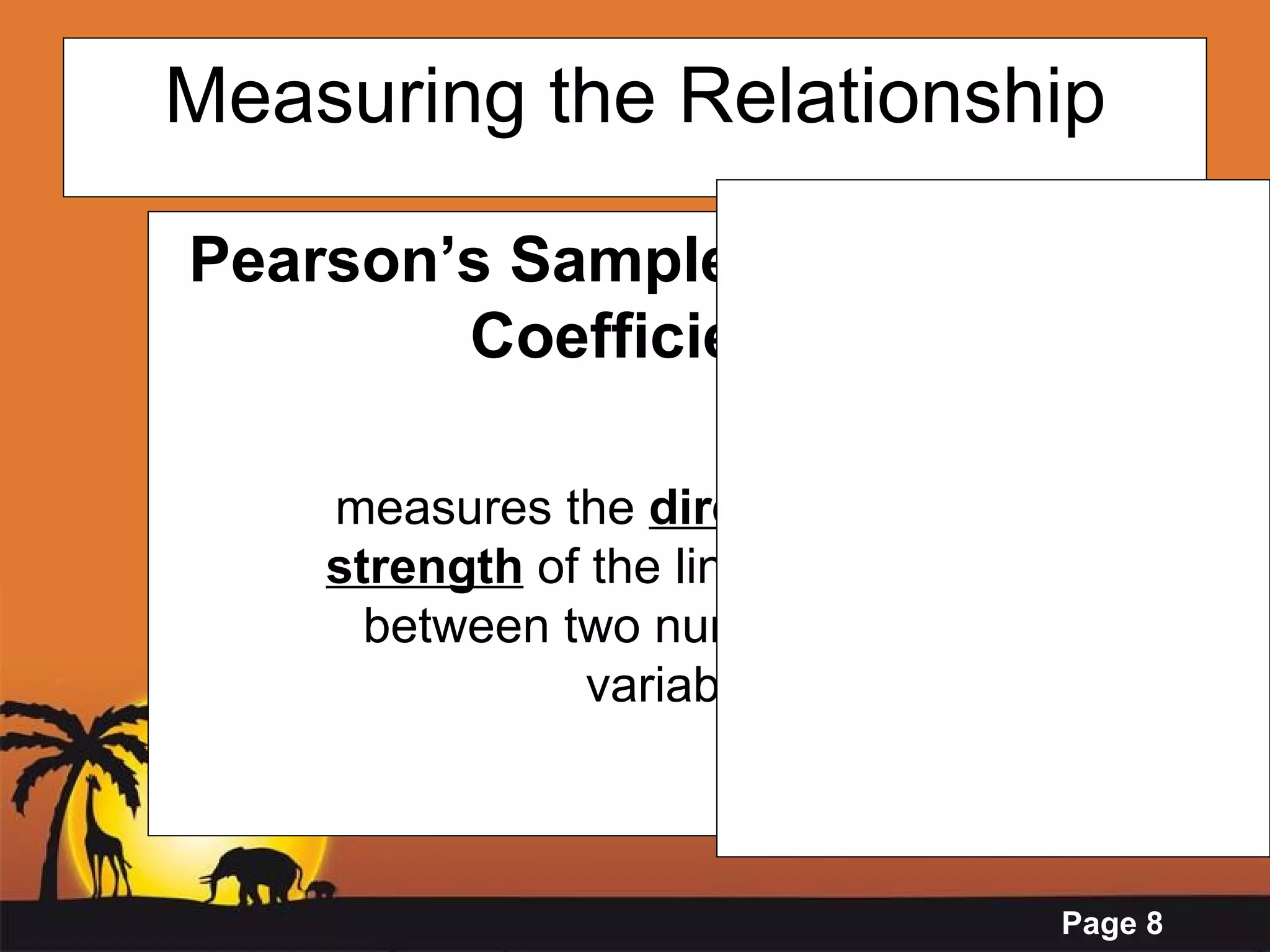
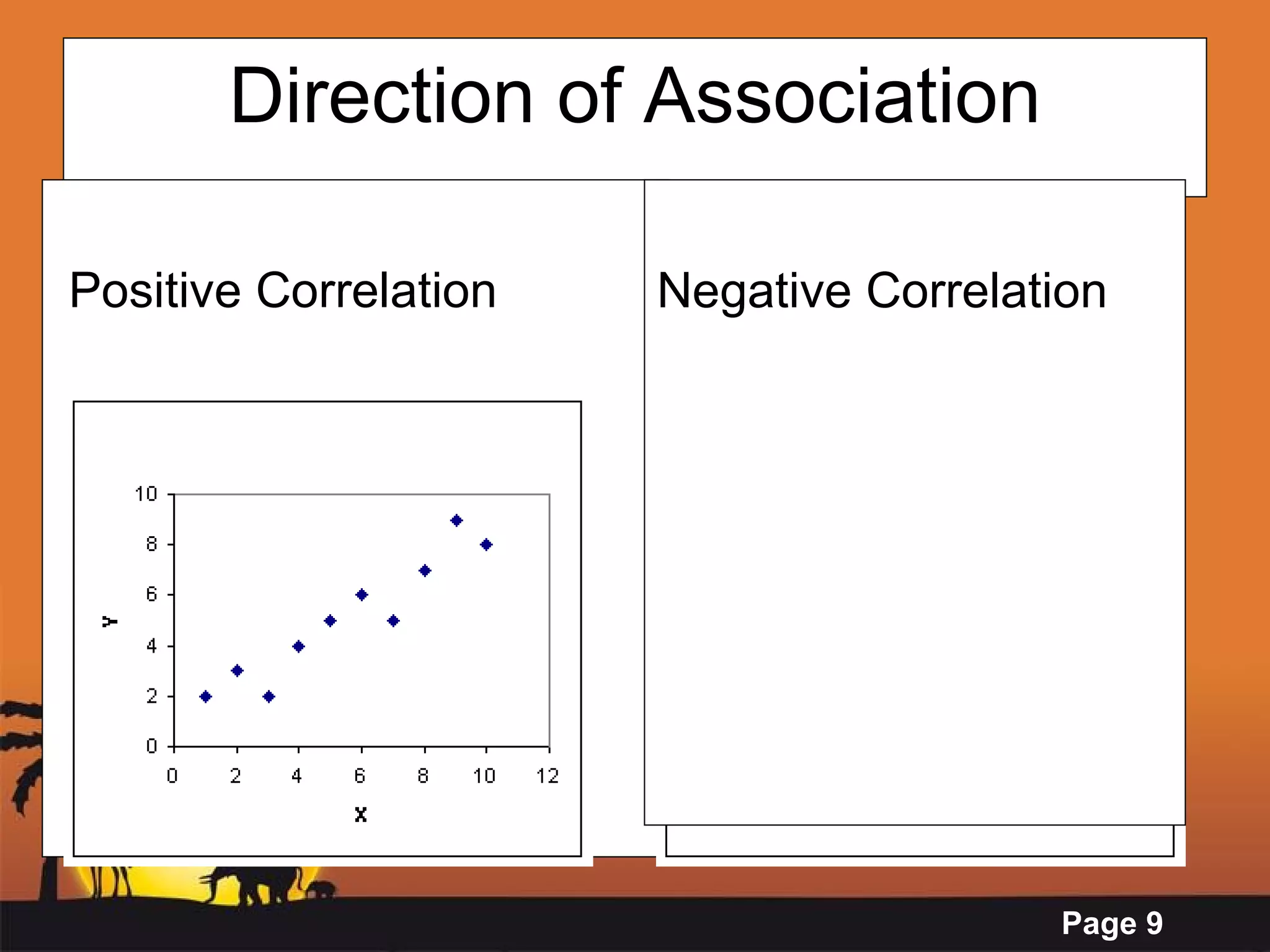
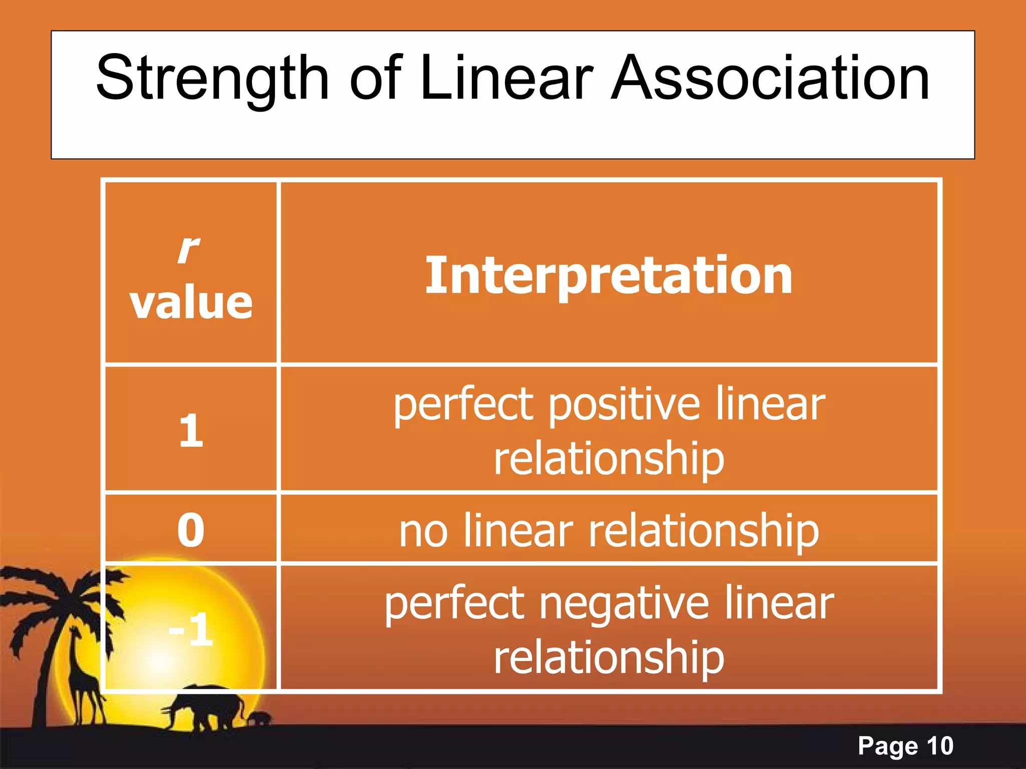
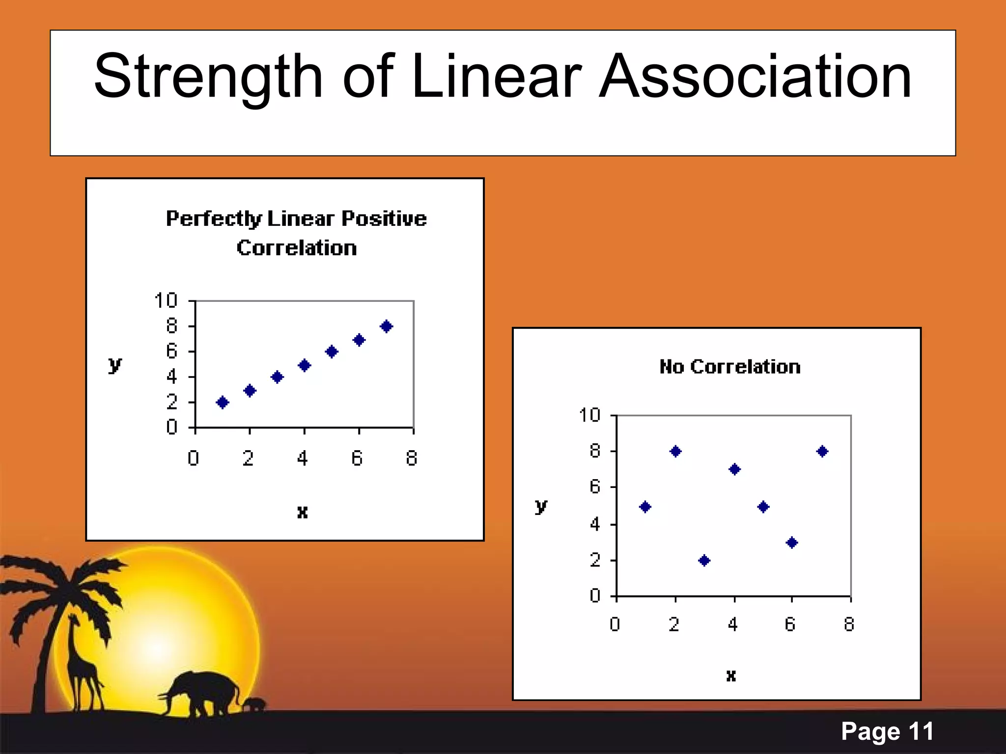
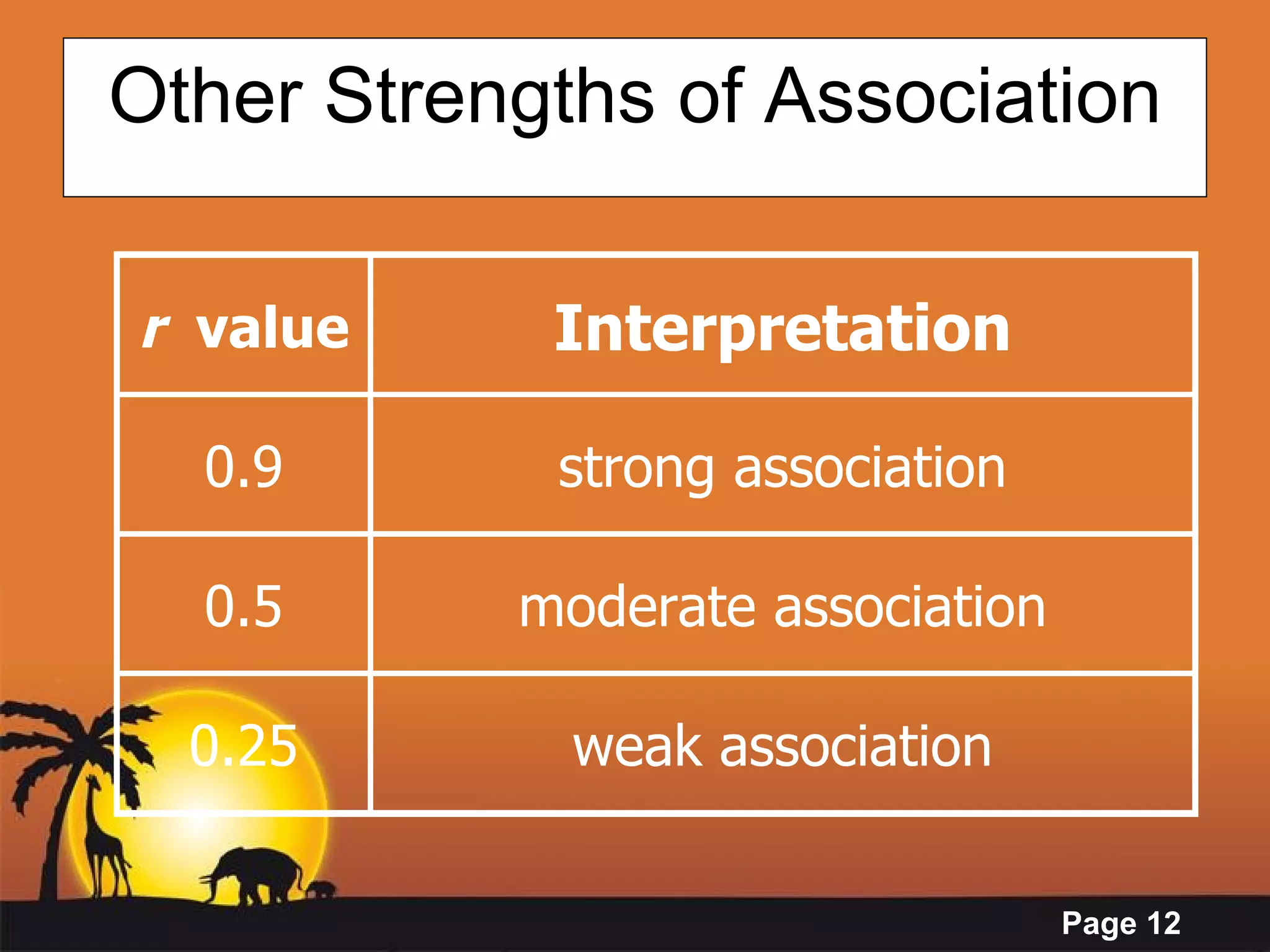
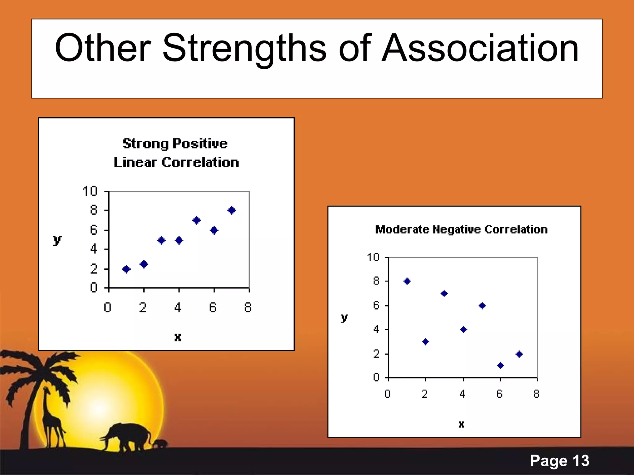
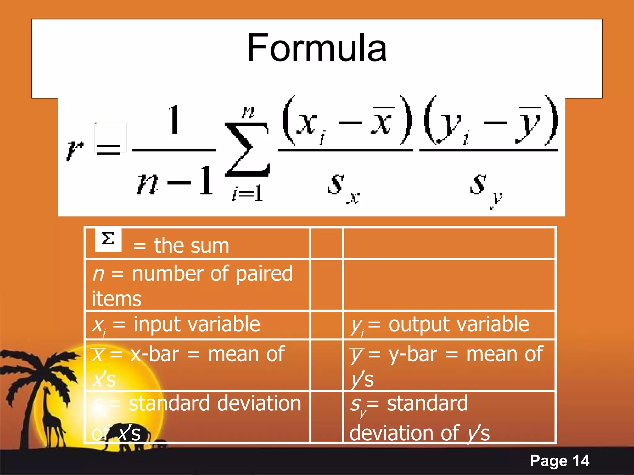
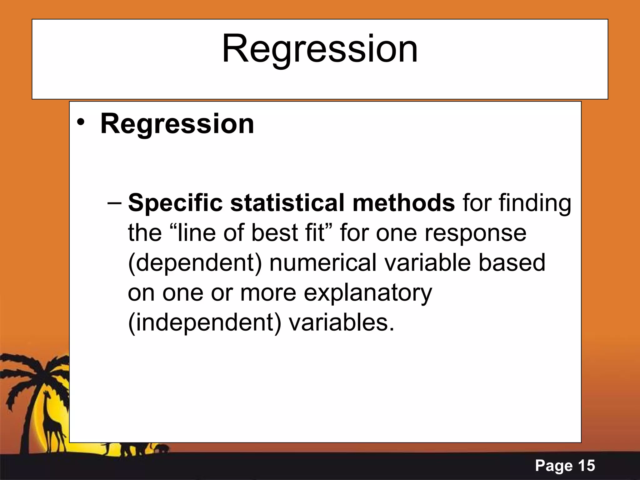
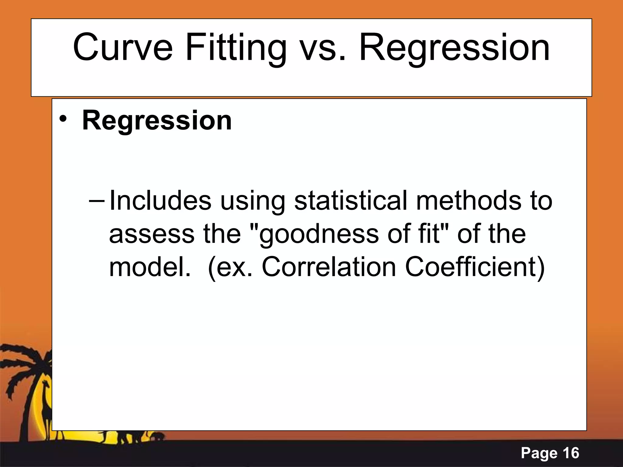
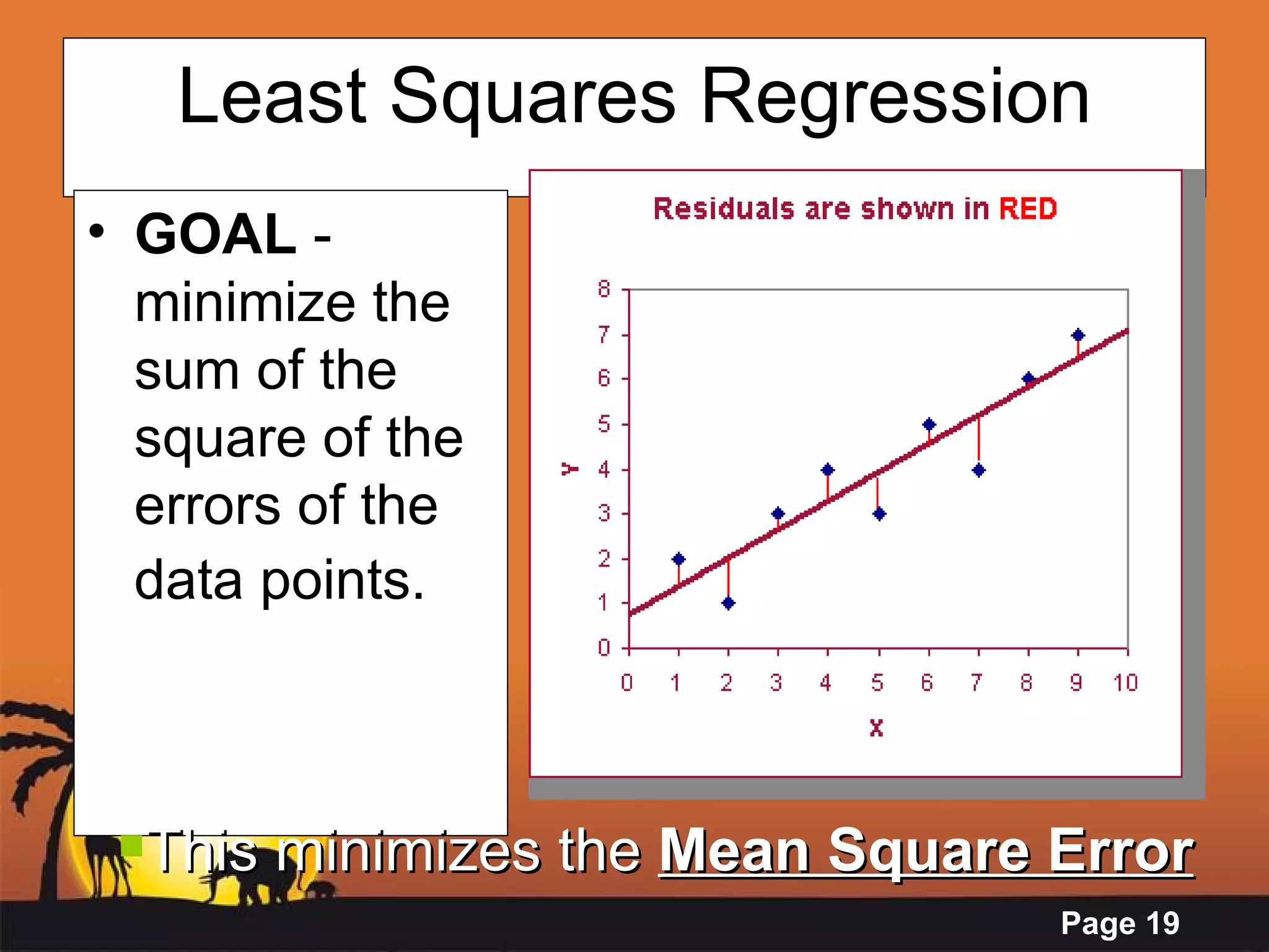
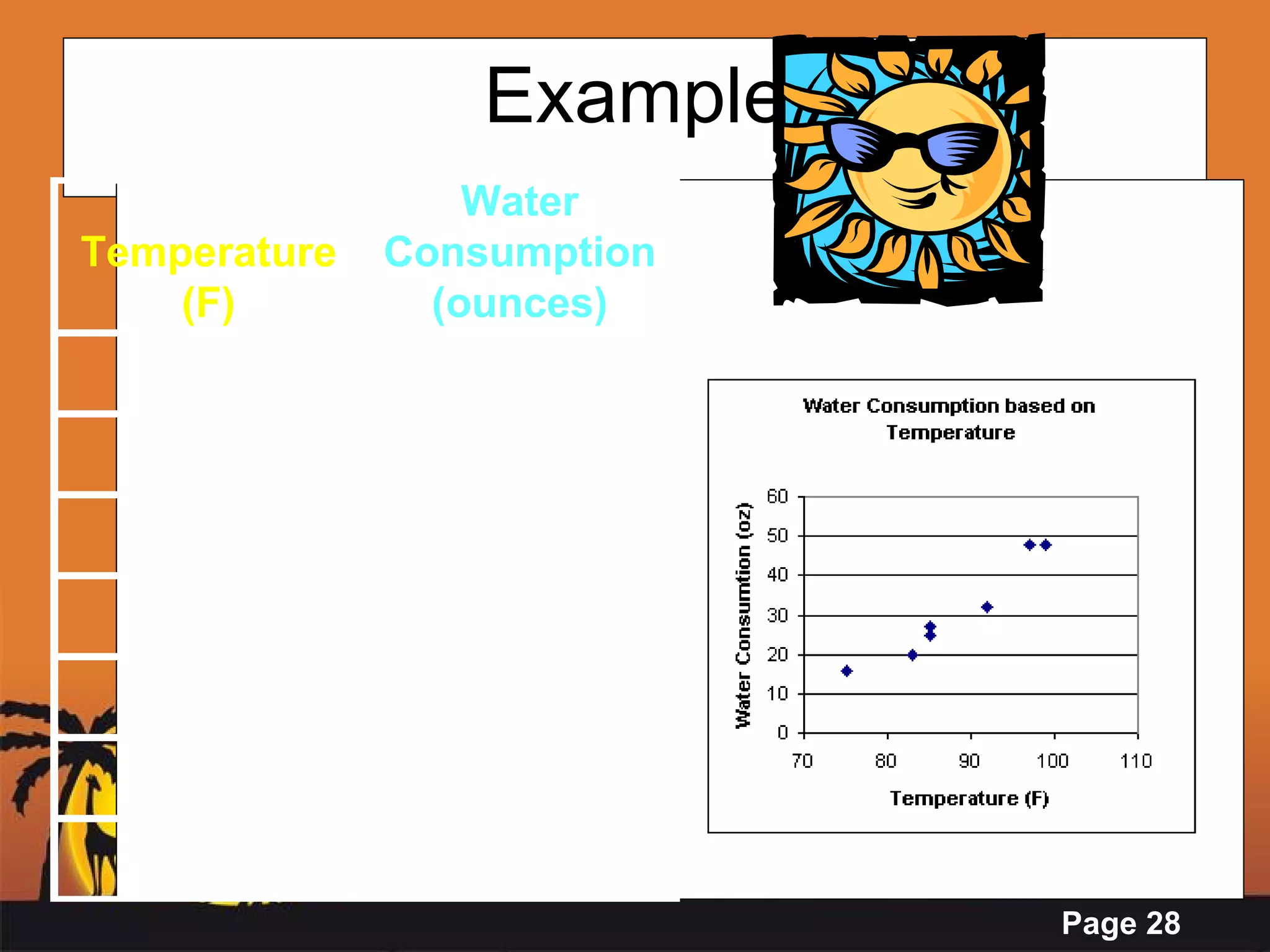
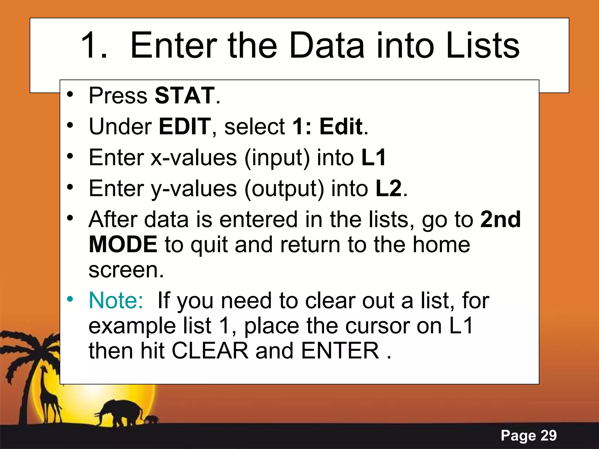
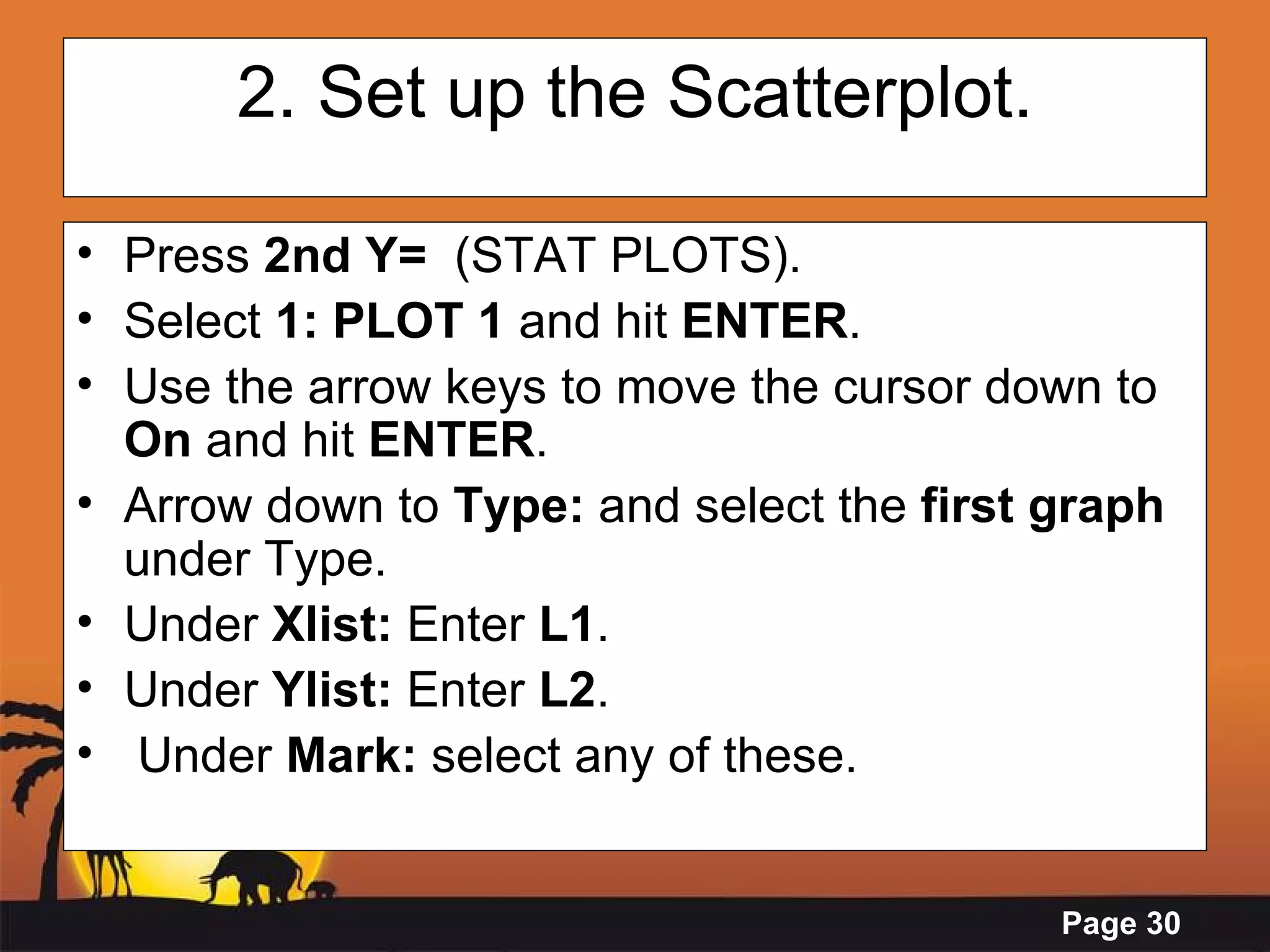
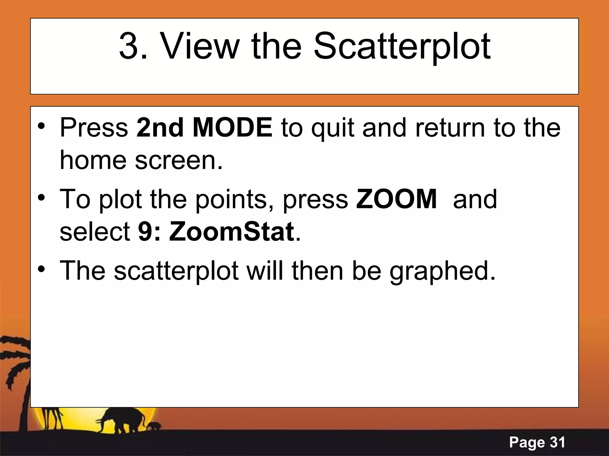
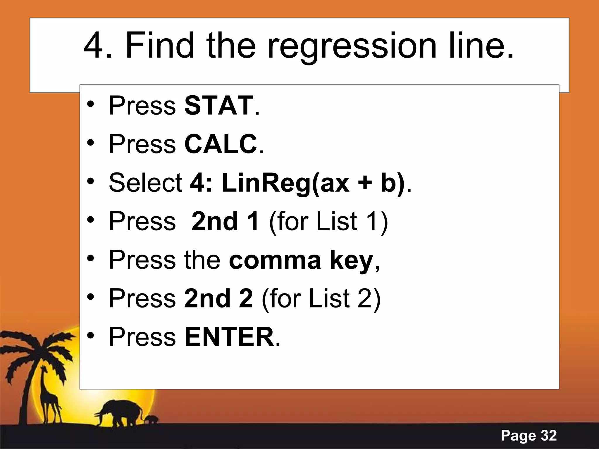
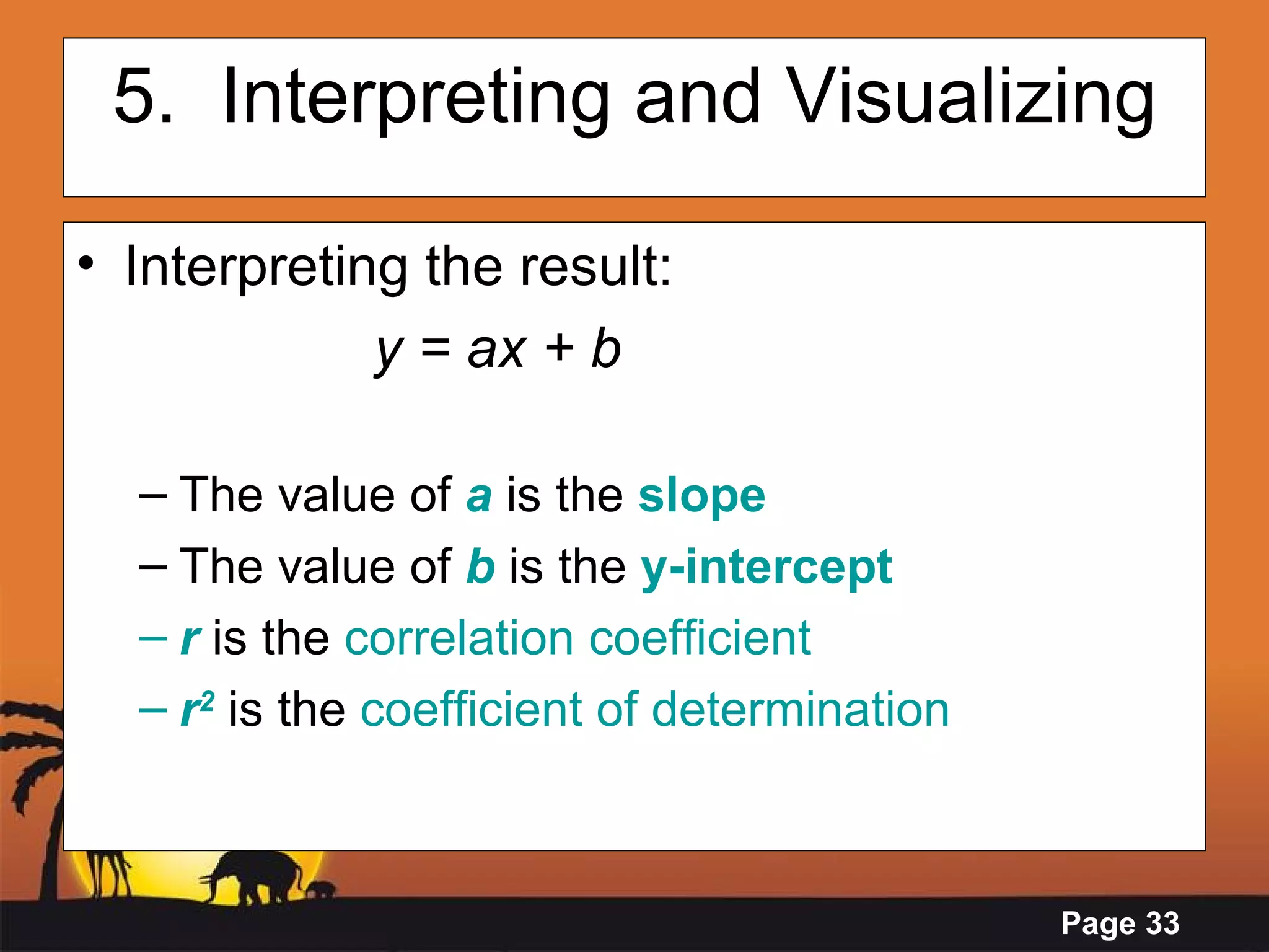


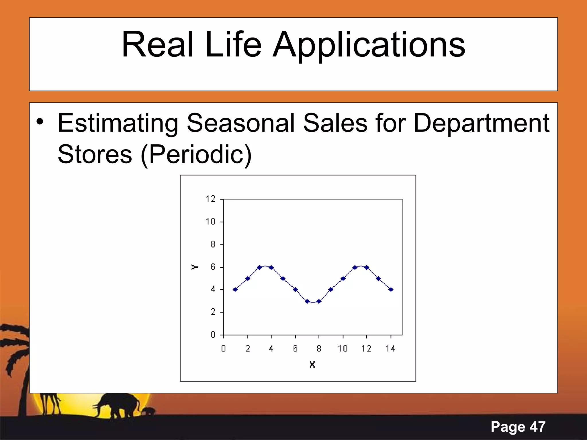

This document provides an introduction to correlation and regression analysis. It defines correlation as a measure of the association between two variables and regression as using one variable to predict another. The key aspects covered are: - Calculating correlation using Pearson's correlation coefficient r to measure the strength and direction of association between variables. - Performing simple linear regression to find the "line of best fit" to predict a dependent variable from an independent variable. - Using a TI-83 calculator to graphically display scatter plots of data and calculate the regression equation and correlation coefficient.