Downloaded 116 times


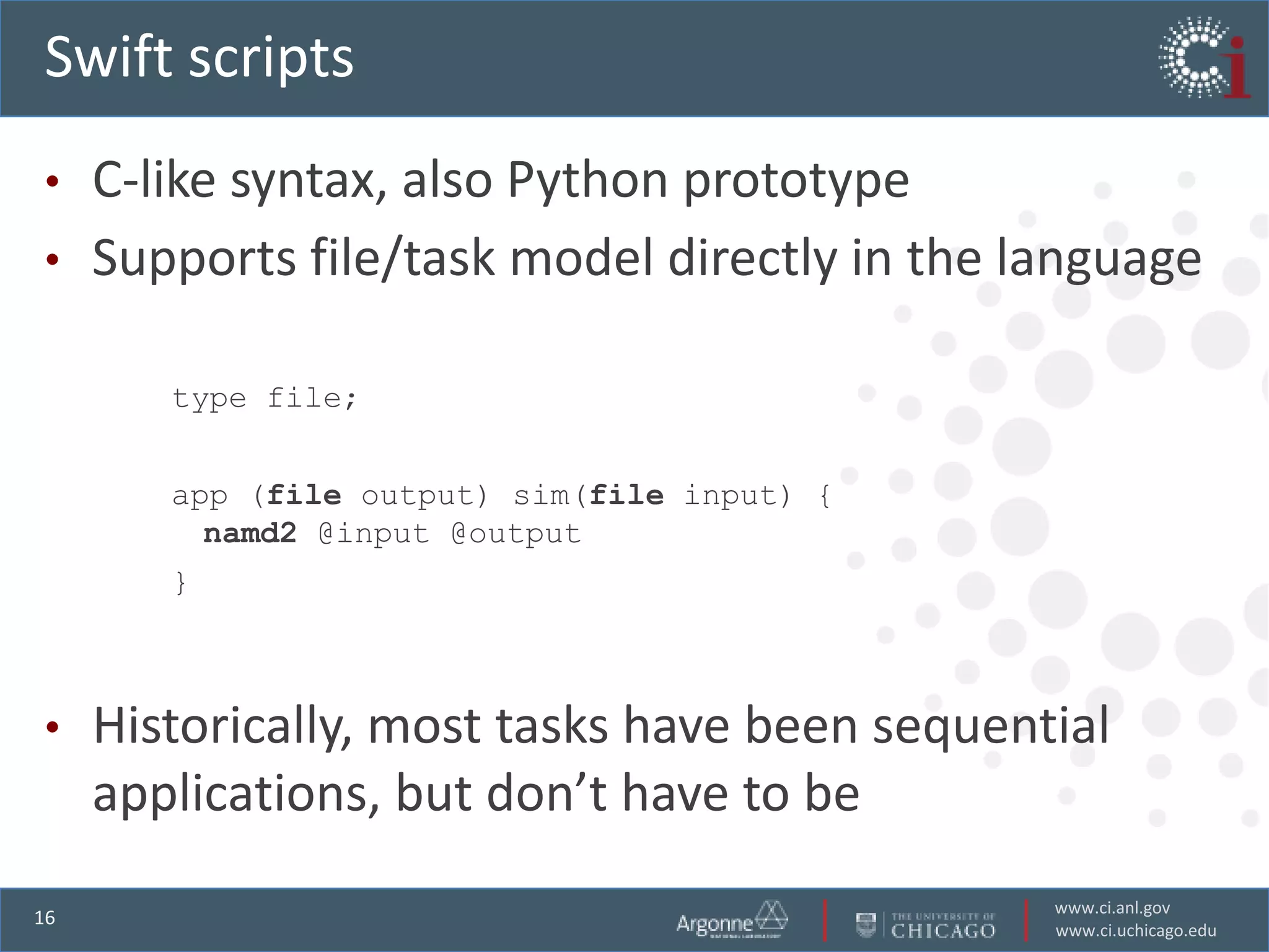
![nSim (1000)
predict()s …
T1af7 T1b72 T1r69
ItFix(p, nSim, maxRounds, st, dt) analyze()
{
...
foreachsim in [1:nSim] {
(structure[sim], log[sim]) = predict(p,st, dt);
}
result = analyze(structure)
...
}
www.ci.anl.gov
21
www.ci.uchicago.edu](https://image.slidesharecdn.com/multiscale-111206062625-phpapp02/75/Multiscale-Modeling-21-2048.jpg)
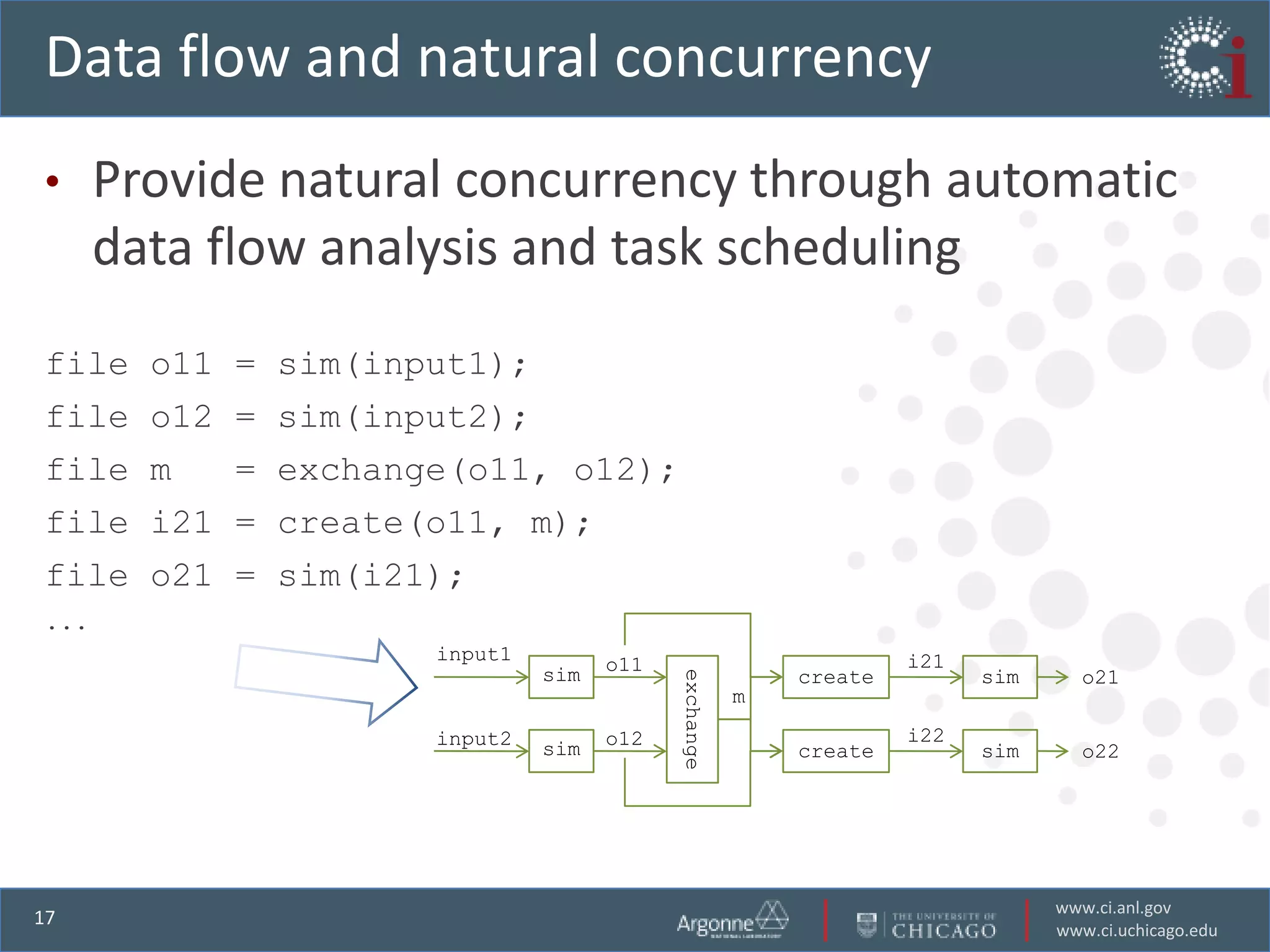
![Powerful parallel prediction loops in Swift
1. Sweep( )
2. {
3. intnSim = 1000;
4. intmaxRounds = 3;
5. Protein pSet[ ] <ext; exec="Protein.map">;
6. float startTemp[ ] = [ 100.0, 200.0 ];
7. float delT[ ] = [ 1.0, 1.5, 2.0, 5.0, 10.0 ];
8. foreachp, pn in pSet {
9. foreacht in startTemp {
10. foreachd in delT {
11. ItFix(p, nSim, maxRounds, t, d);
12. }
13. }
14. }
15. }
10 proteins
x 1000 simulations x
3 rounds x 2 temps x 5 deltas
= 300K tasks
www.ci.anl.gov
22
www.ci.uchicago.edu](https://image.slidesharecdn.com/multiscale-111206062625-phpapp02/75/Multiscale-Modeling-22-2048.jpg)
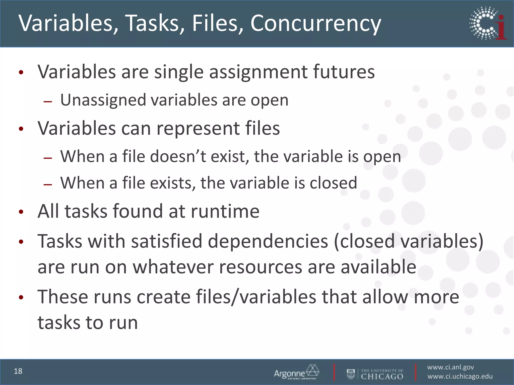
![Swift code
//Hybrid Model
(file simOutput) HybridModel (file input) {
// Driver …
file stompIn<"stomp.in">; stompOut = runStomp(input);
iterate iter { (sphins, numsph) = pg(stompOut, sphinprefix);
output = HybridModel(inputs[iter]);
inputs[iter+1] = output; //Find number of pore scale runs
capture_provenance(output); intn = @toint(readData(numsph));
foreachi in [1:@toint(n)] {
} until(iter>= MAX_ITER); sphout[i]= runSph(sphins[i], procs_task)
}
simOutput = gpg(sphOutArr, n, sphout);
}
Credit: Karen Schuchardt , Bruce Palmer, KhushbuAgarwal, Tim Scheibe, PNNL
www.ci.anl.gov
37
www.ci.uchicago.edu](https://image.slidesharecdn.com/multiscale-111206062625-phpapp02/75/Multiscale-Modeling-37-2048.jpg)


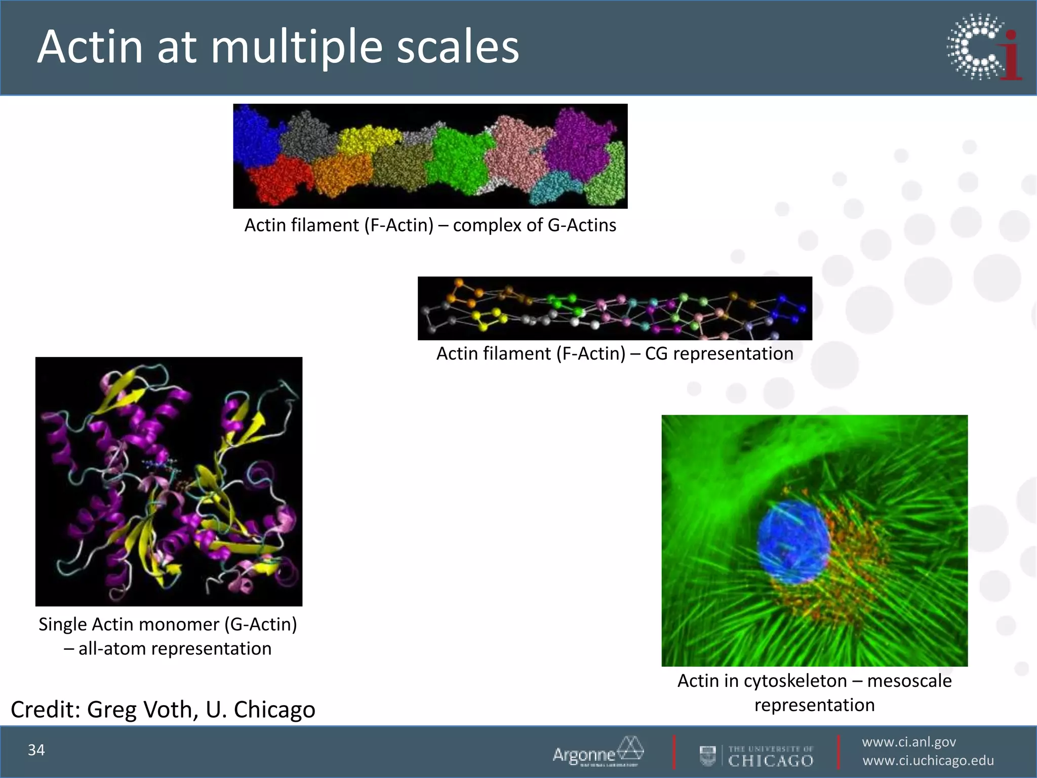
The document discusses the development of multiscale modeling tools by the Computation Institute to address complex scientific problems through strategic computation. It emphasizes the importance of coupling multiple models across different scales in material science and computational biology to predict phenomena accurately. The institute aims to create effective computational tools and educate the next generation of researchers to enhance multidisciplinary collaborations and discoveries.
Overview of multiscale modeling tools presented by Daniel Katz at the Computation Institute.
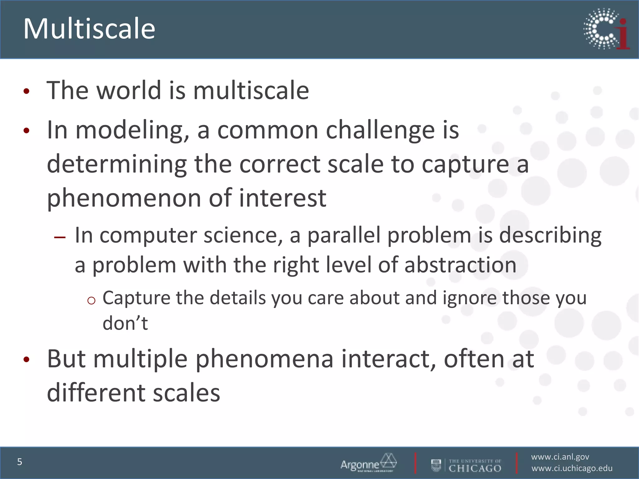
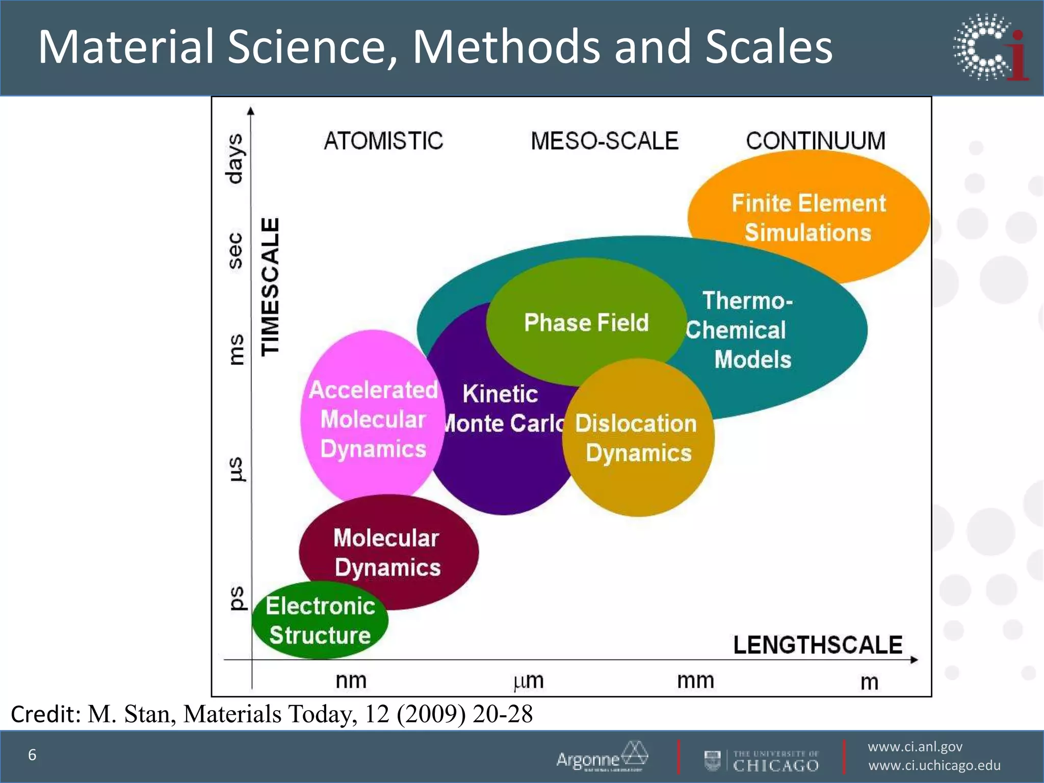
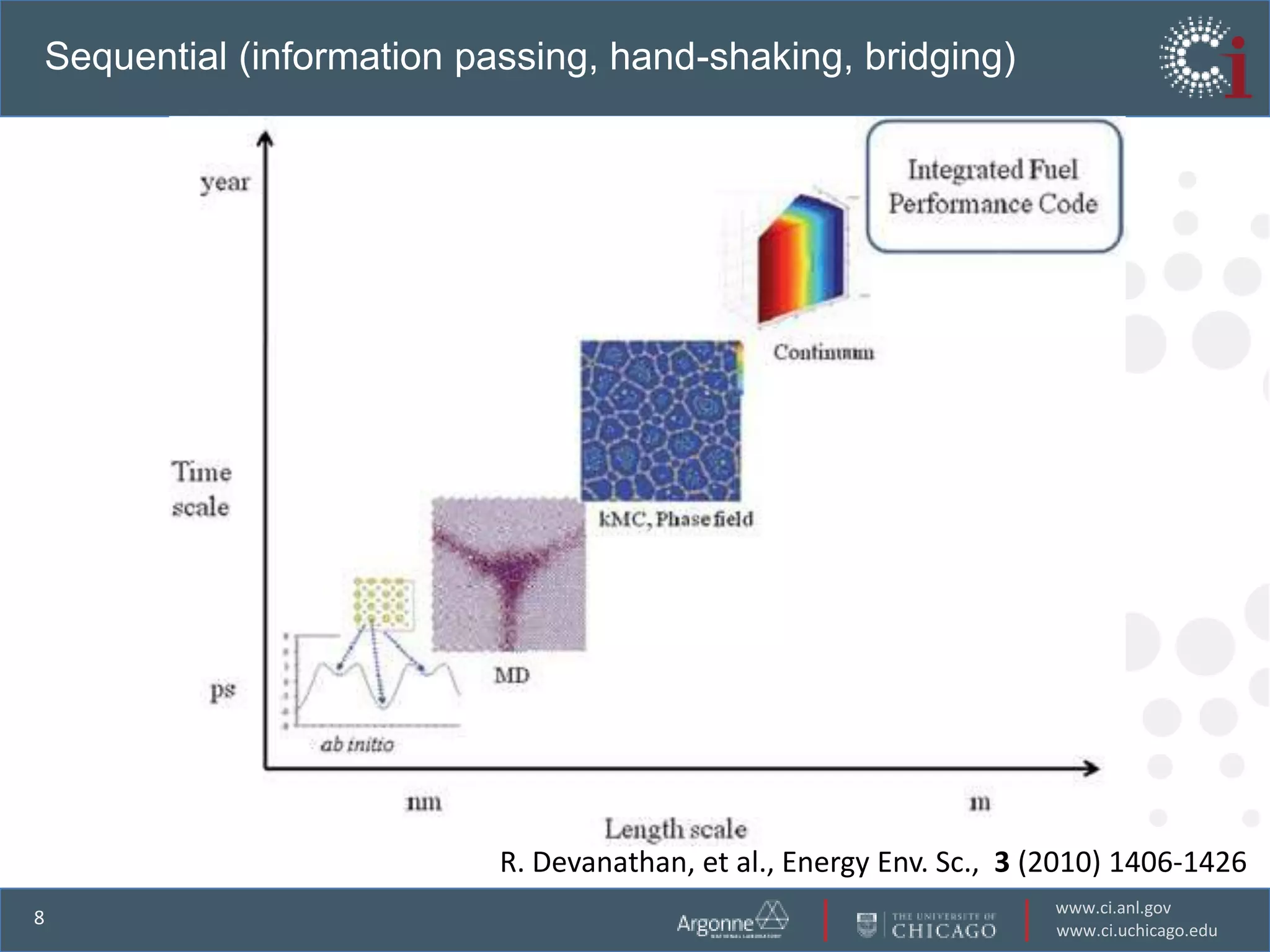
Introduction to multiscale concepts and their application in modeling, especially in material science.
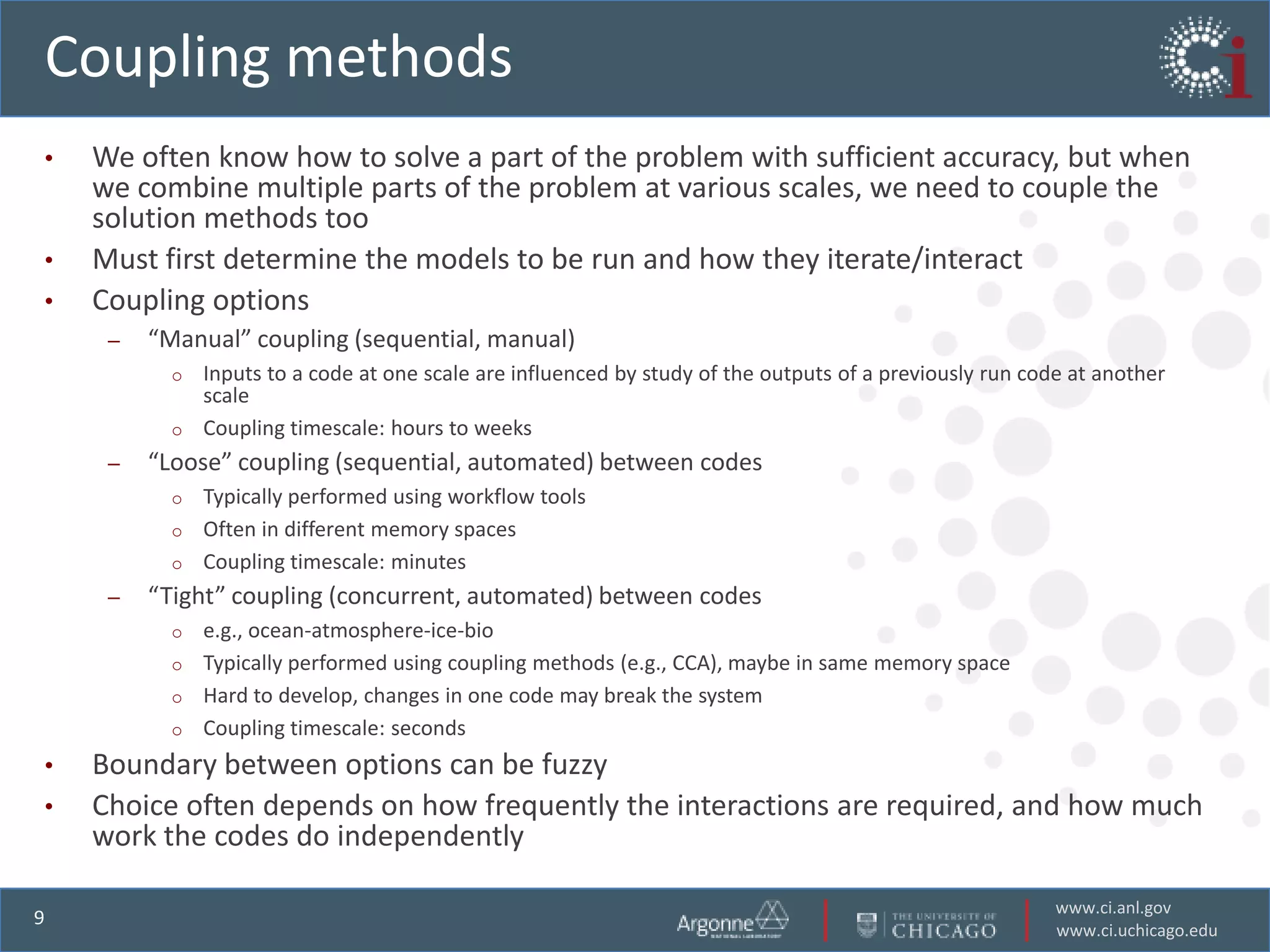
Describes specific challenges faced in multiscale modeling such as material modeling and solution coupling methods.
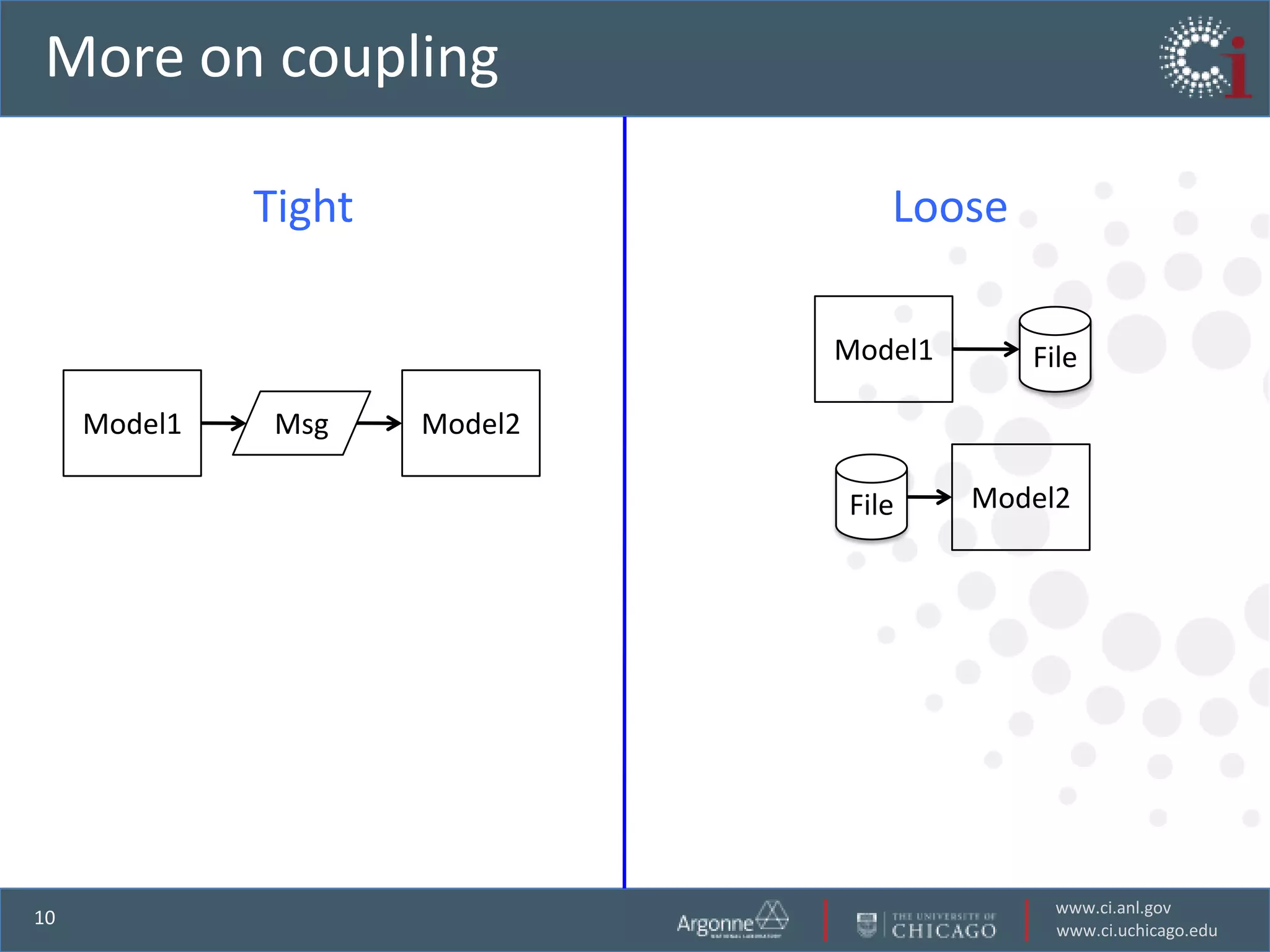
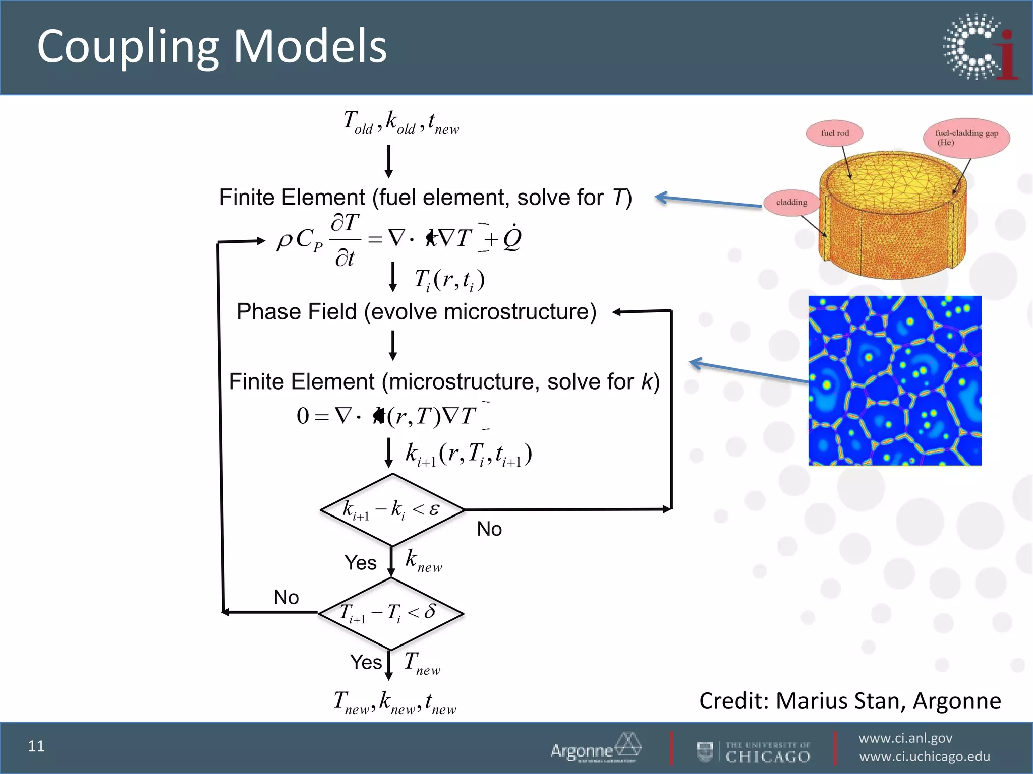
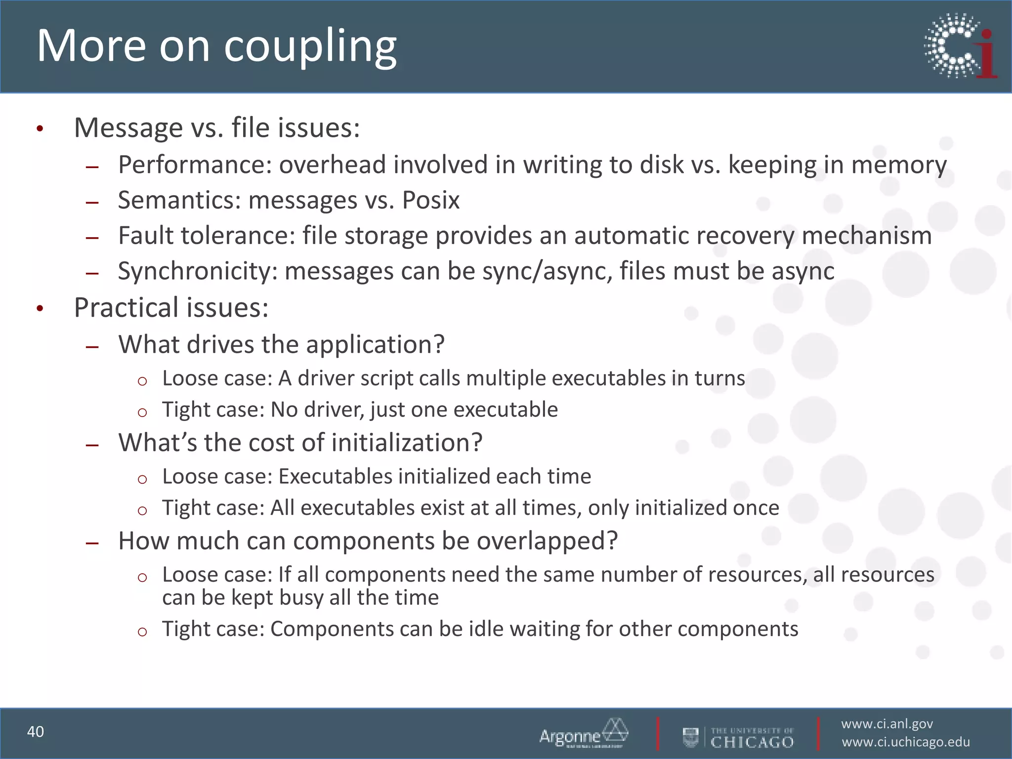
Explains different coupling strategies in multiscale models: tight, loose, and sequential coupling.
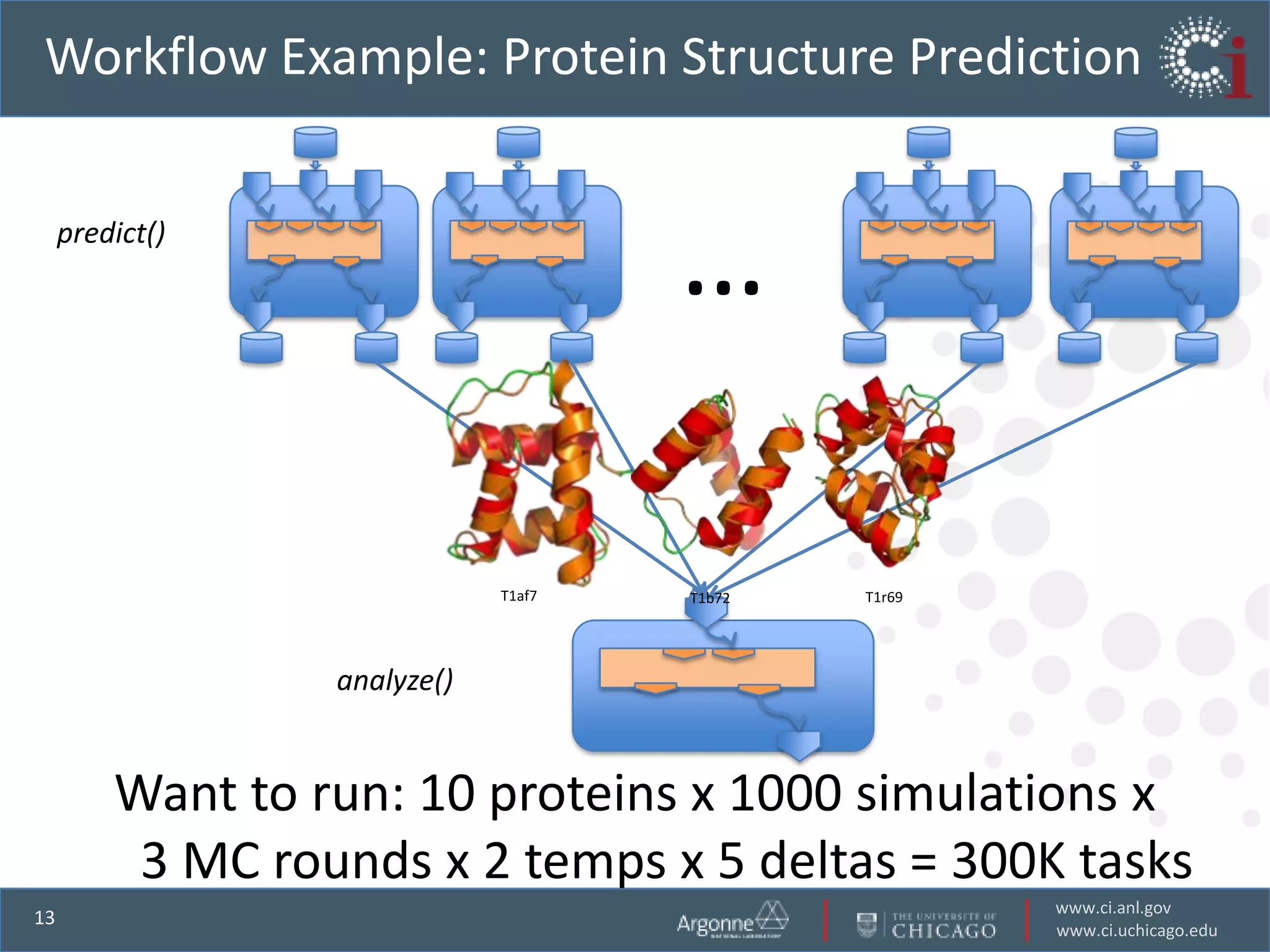
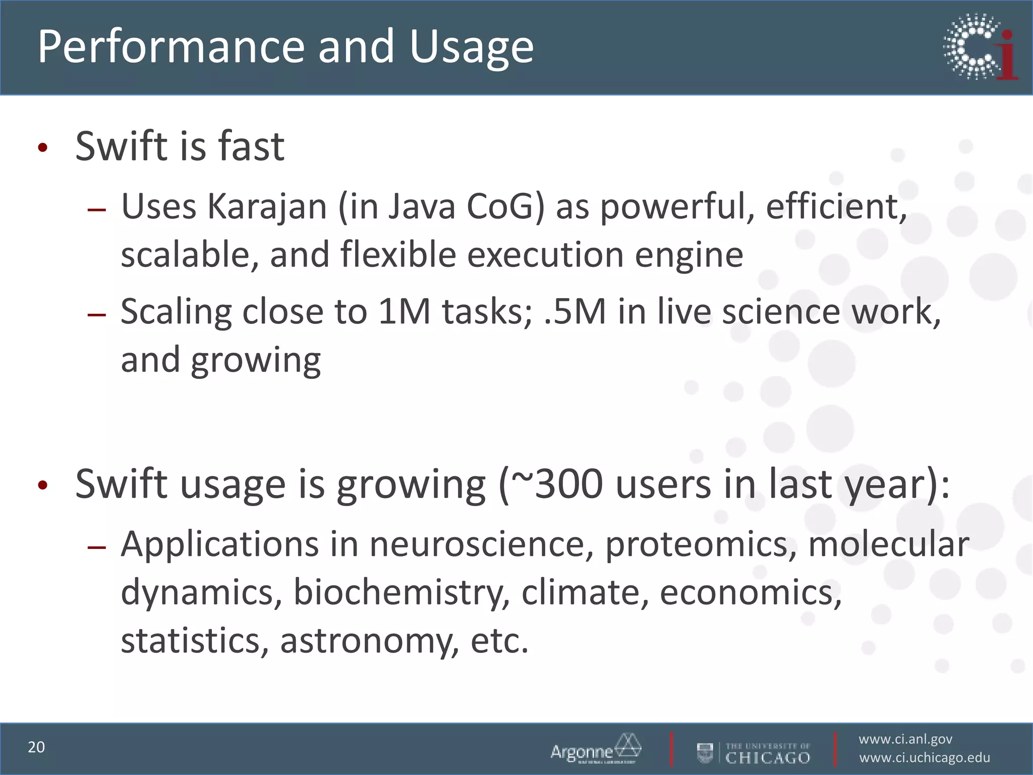
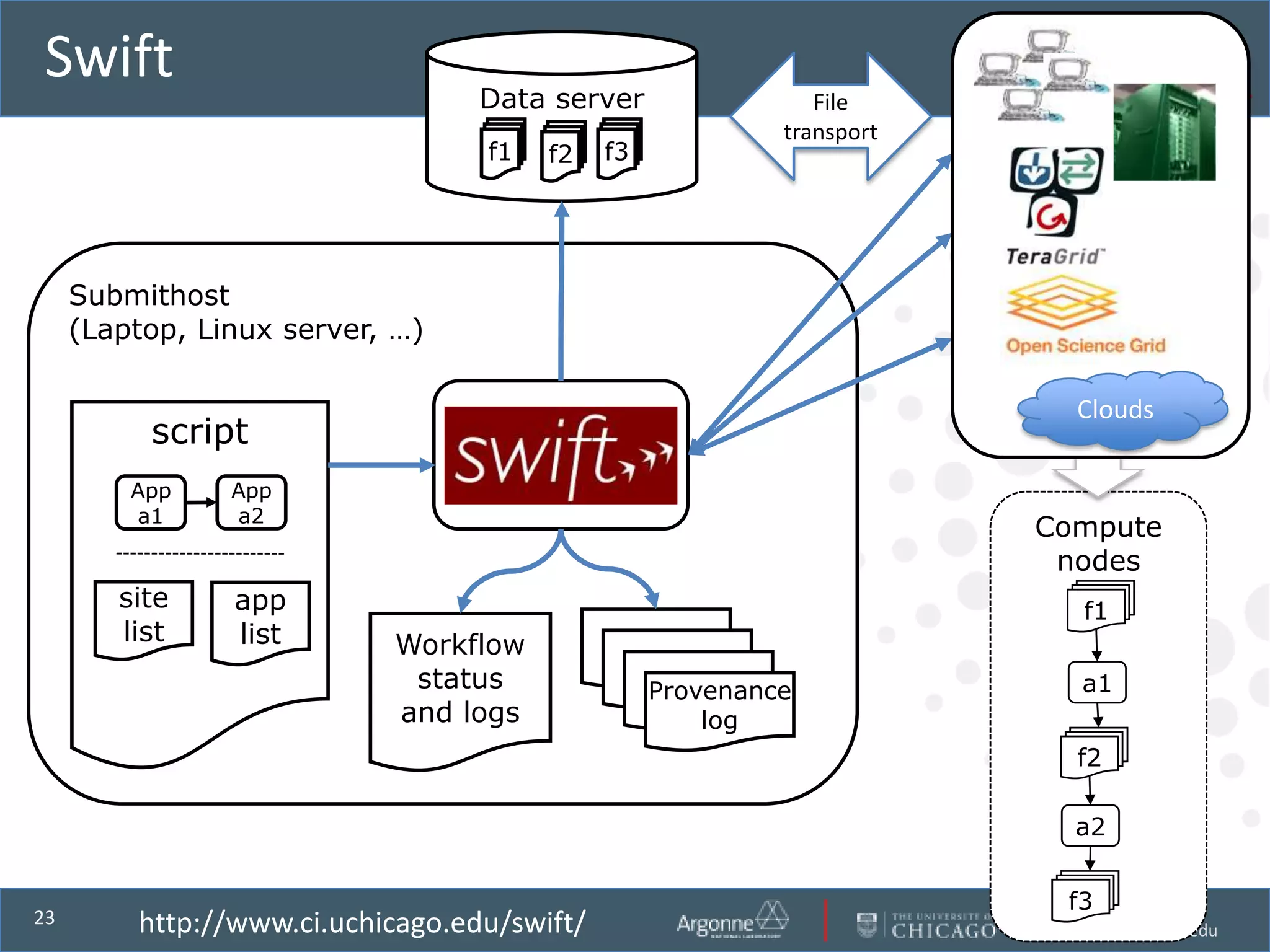
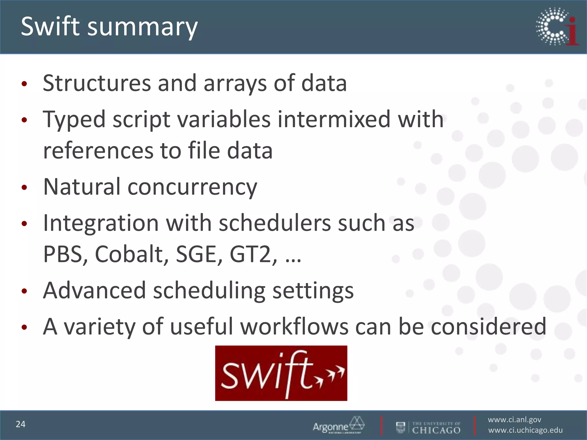
Presents Swift as a tool for managing workflows in multiscale modeling with examples of complex tasks.
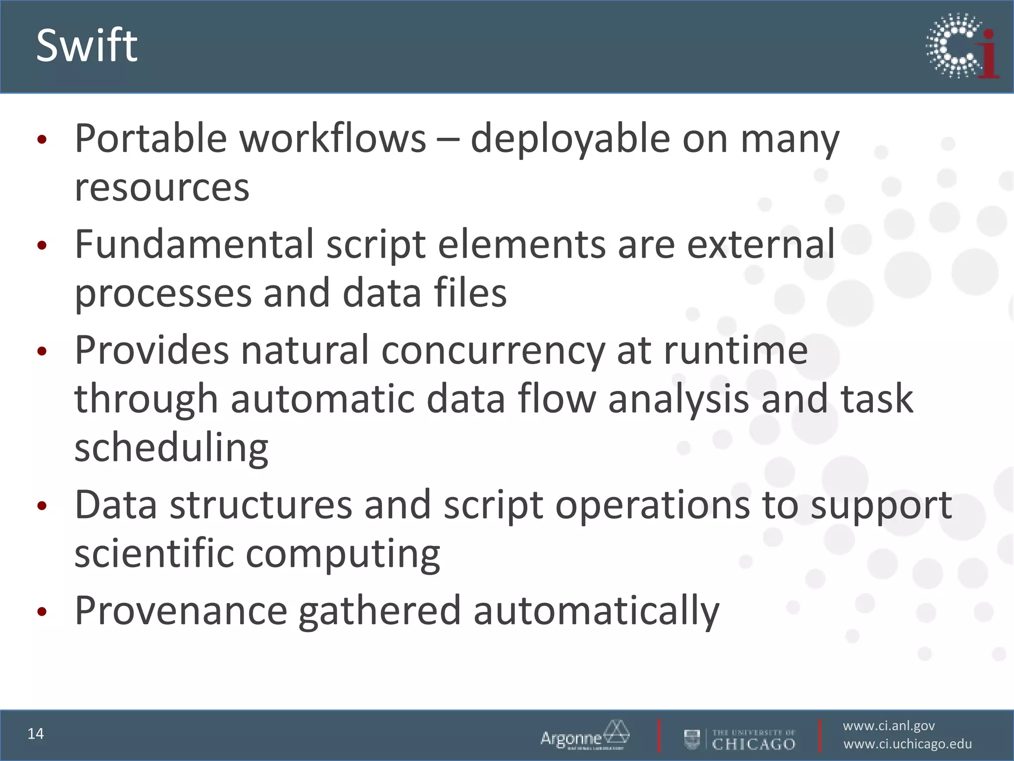
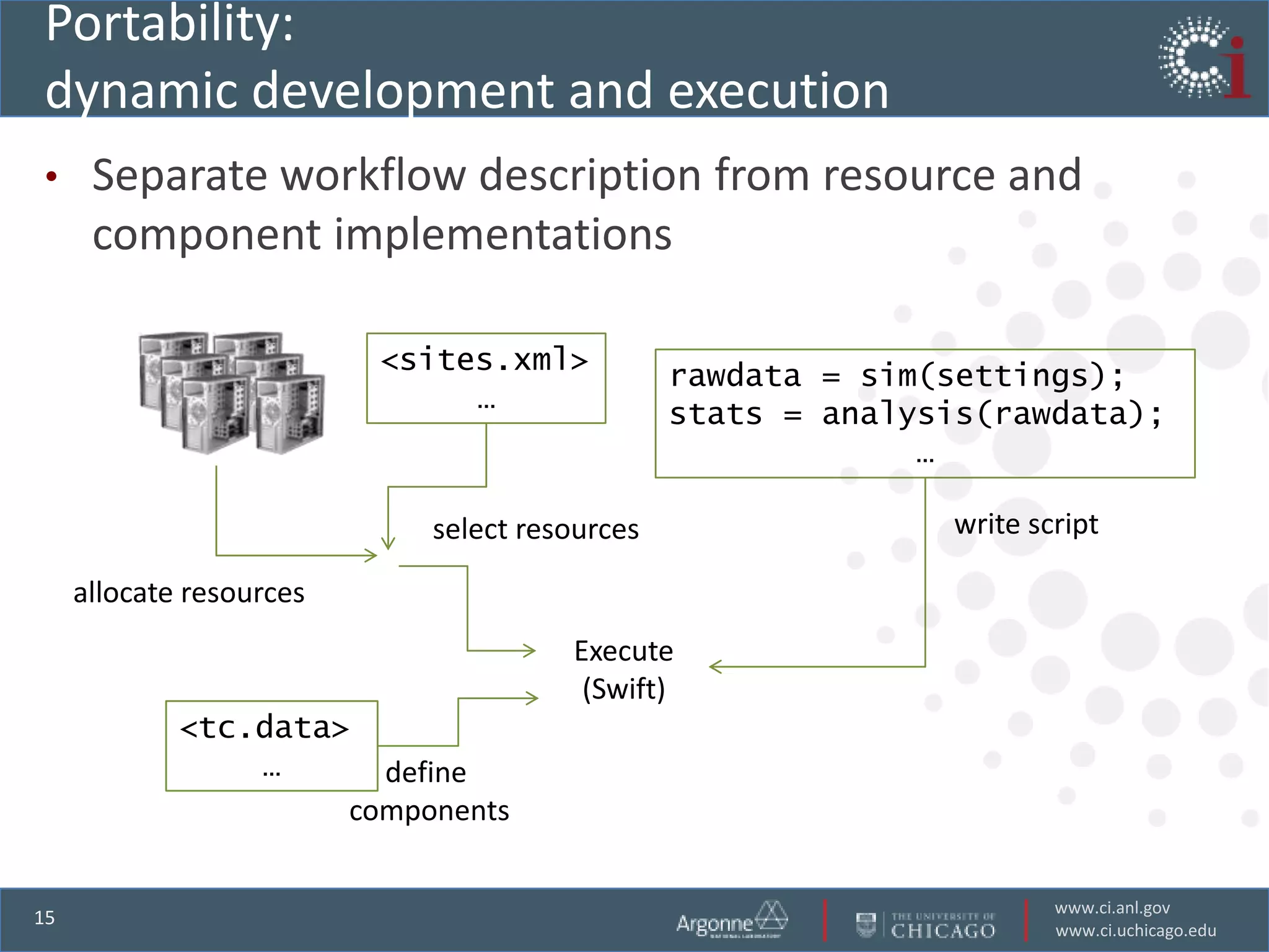
Details Swift's capabilities, performance metrics, and growth in applications across various fields.
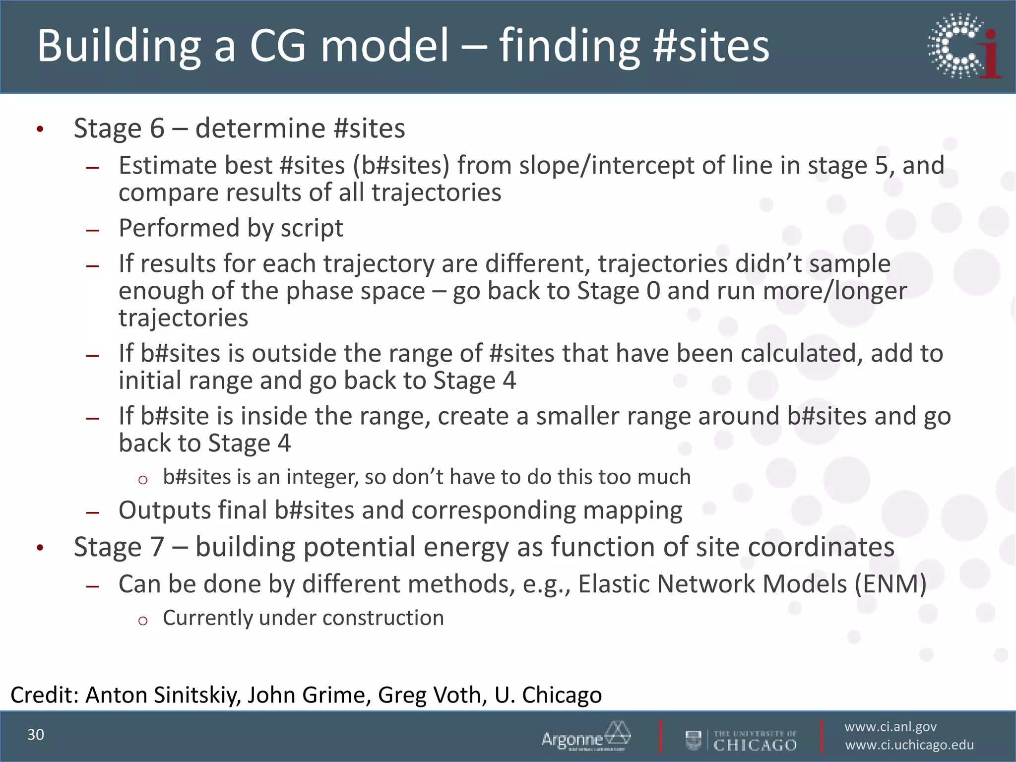
Focuses on creating coarse-grained models and outlines the multi-stage process involved.
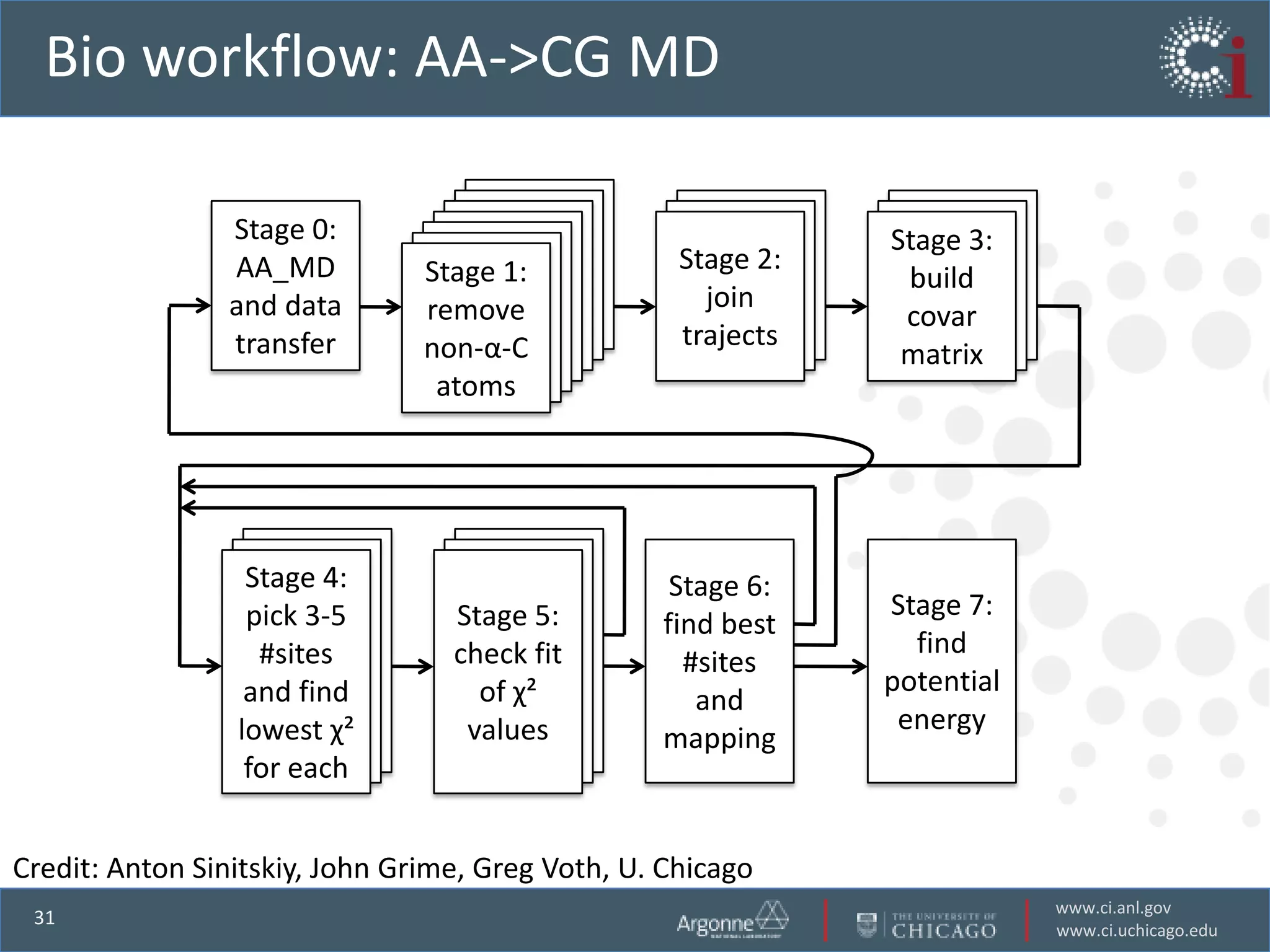
Describes the bio workflow from all-atom (AA) to coarse-grained (CG) modeling in biological systems.
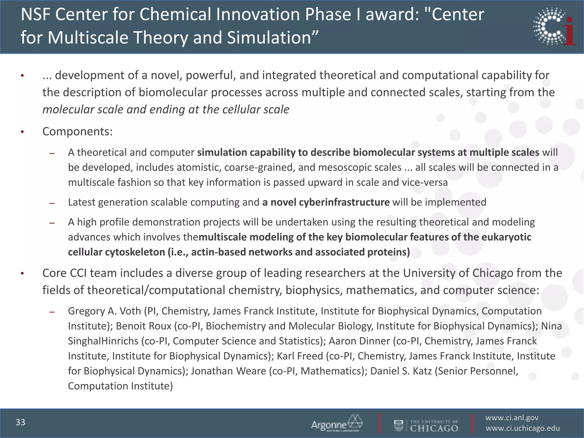
Presents NSF's Center for Multiscale Theory emphasizing connections from molecular to cellular scales.
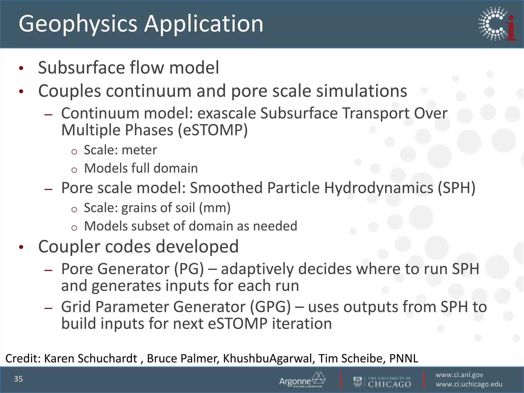
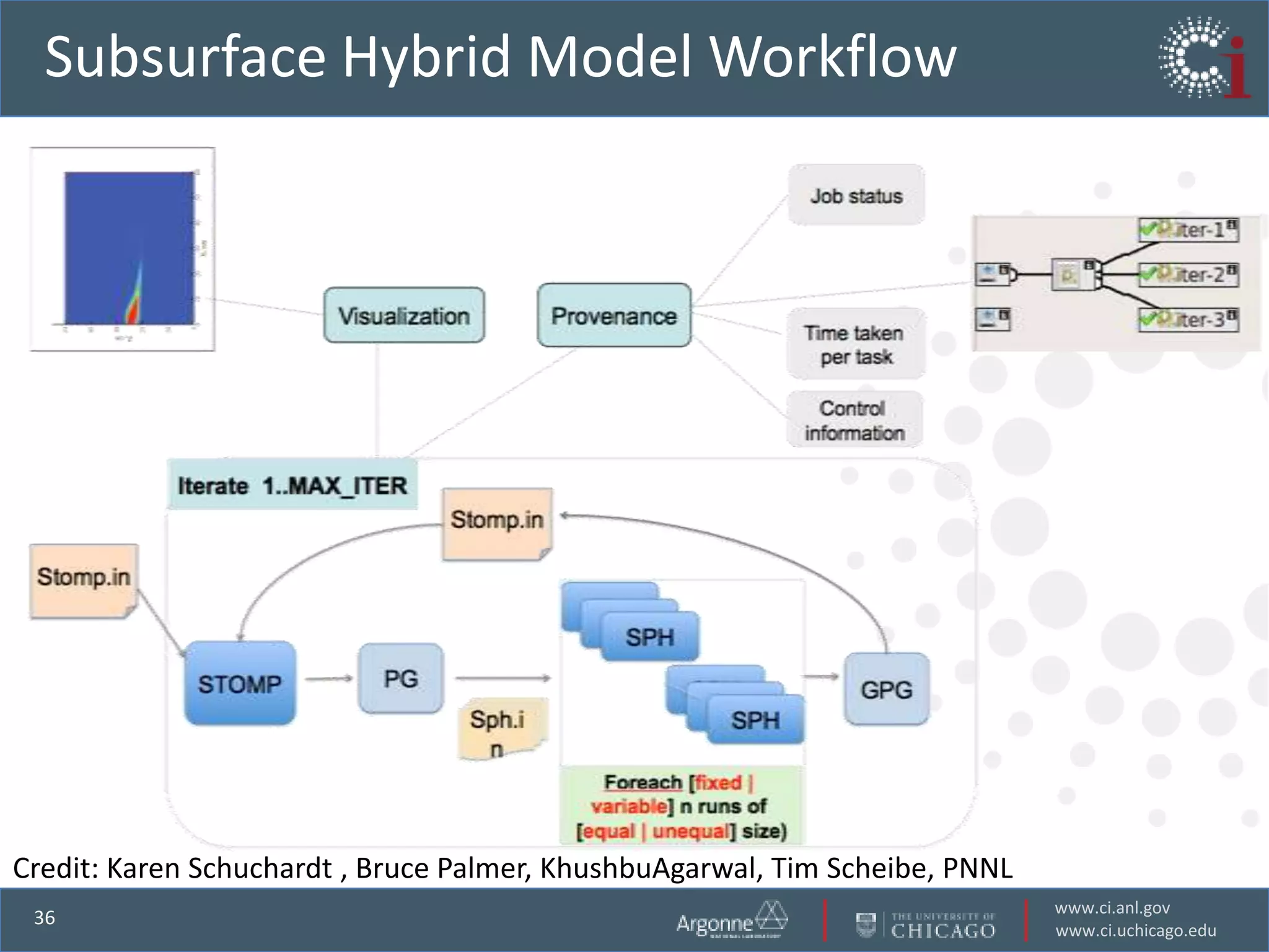
Discussion on subsurface flow models, coupling continuum, and pore scale simulations.
Details a hybrid model using Swift for creating complex task workflows in geophysics.
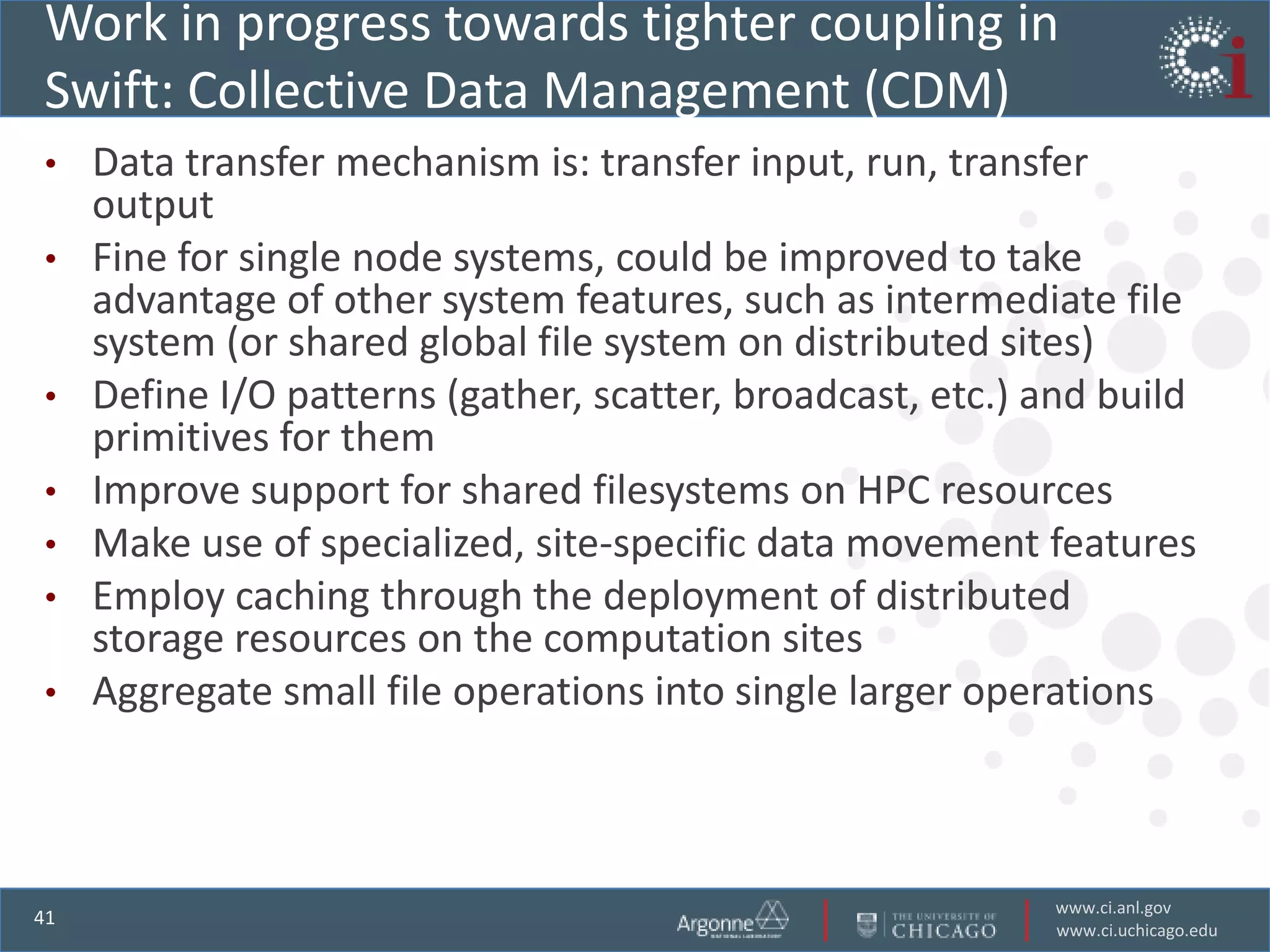
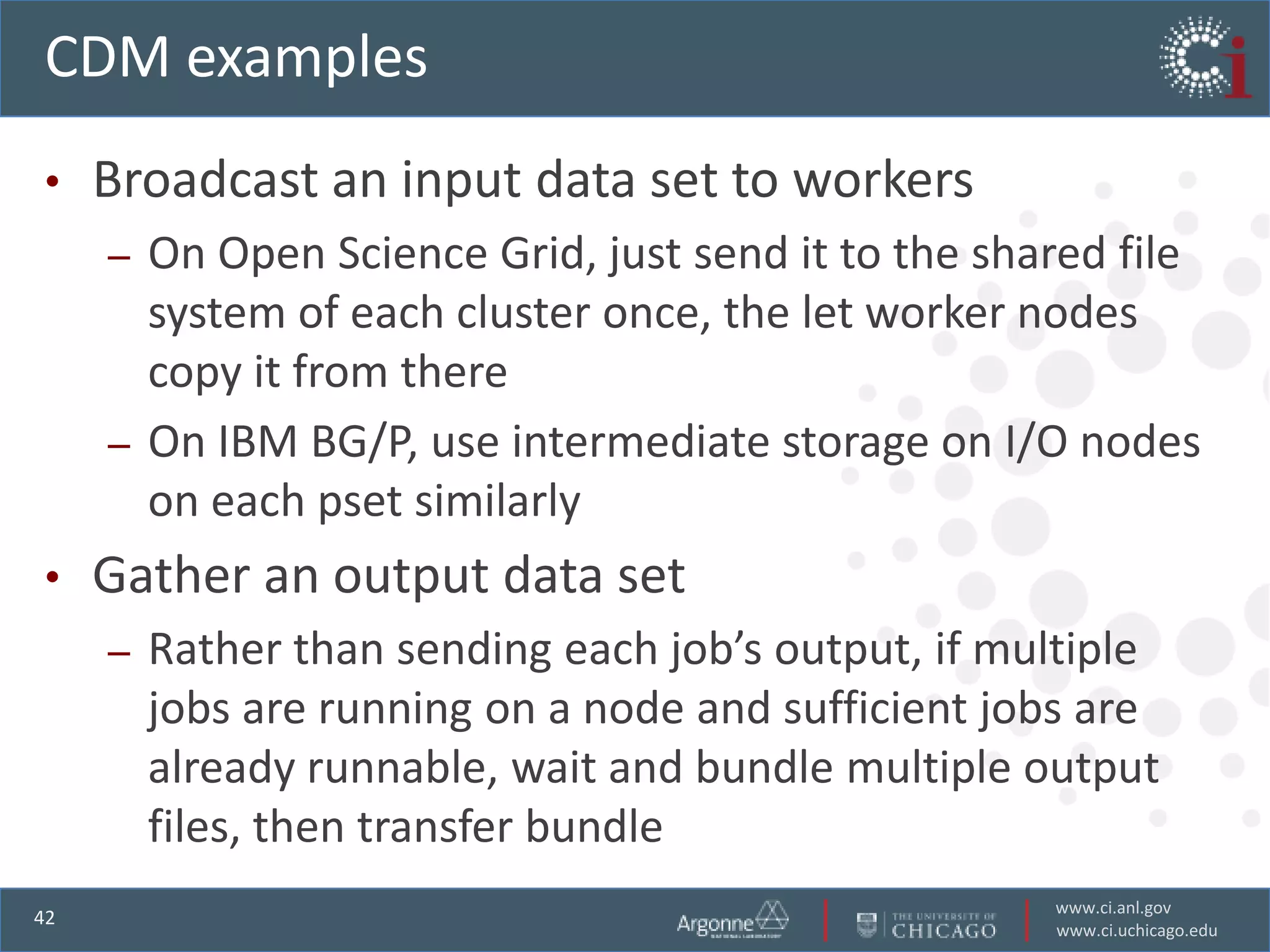
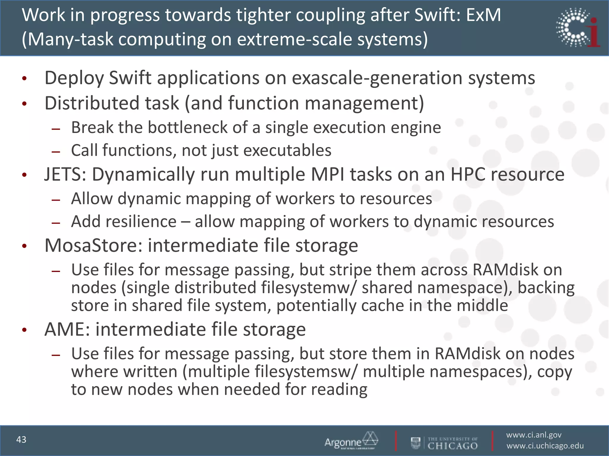
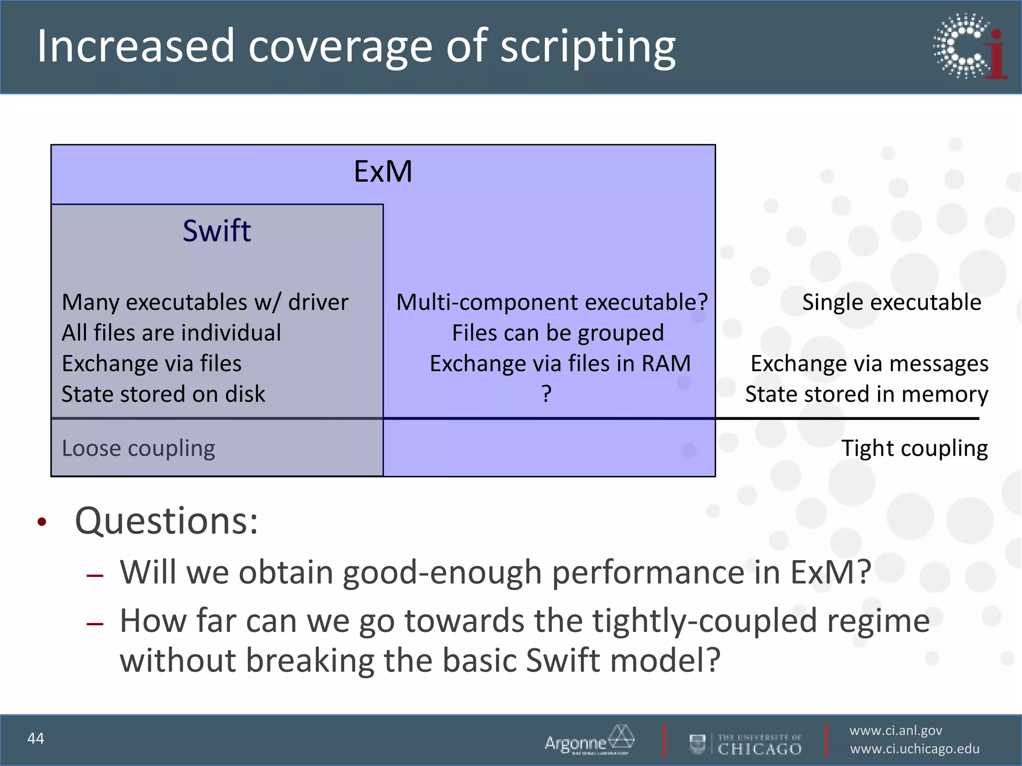
Conclusion on the movement towards tighter coupling in multiscale modeling using Swift.
Acknowledges support from various organizations and contributors involved in Swift and ExM.