Chapter 17 Cost Variance Analysis • 16–3 Learning Objectives •  Describe what is meant by cost control. •  Describe the two major theories used for the detection of out of control costs. •  Define variance analysis and how it is used by management. •  Calculate the various types of cost variances. •  Explain and calculate price, efficiency and volume variances. 2 Figure 17-1: Phases of Cost Control Efficiency Cost •  Total cost that results from an out of control situation •  Efficiency Cost Equals –  T x R x P –  T = Total time from problem occurrence to correction –  R = Loss or cost per time unit –  P = Probability that problem can be corrected • 16–5 4 Alternatives for Minimizing Efficiency Cost •  Preventive Approach –  Minimize P (Probability of a problem occurring) –  Emphasis on right people with right motivation •  Detection-Correction Approach –  Minimize T (Total time problem is present) –  Emphasis on reporting and variance analysis • 16–6 5 • 16–7 Variance Analysis Requirements for variance analysis •  Standards (budgets) •  Related cost accounting system •  Fixed/variable split of costs Phases in cost control •  Recognition of problem •  Determination of cause •  Correction o Budgetary o Operational 6 Alternative Methods to Determine when to Investigate a Variance • 16–8 • Control Chart - Biggest problem is failure to recognize costs of investigation or benefits of problem correction x = 0 x + 2σ x - 2σ 7 Alternative Methods (cont.) •  Decision Theory (Payoff Table) –  I = Cost of Investigation –  L = Loss if system out of control • 16–9 8 Alternative Methods (cont) •  Variances should be investigated if the probability that the system is in control is less than: •  Example – –  I = $1,000 –  L = $4,000 –  Investigate when probability of system being in control is less than 75% • 16–10 1.0 - Cost of Investigation (I) Loss if out of control (L) 9 Variance Analysis Areas •  Facility Level –  High level explanation of why costs have changed •  Departments/Responsibility Centers –  Prior period cost analysis –  Budgetary cost comparisons •  Health Plan/Managed Care • 16–11 10 • 16–12 Variance Analysis—Facility Level Cost per discharge changes result from •  Resource price changes •  Productivity changes •  Intensity changes Cost Equation •  CPD = •  Ci = Cost (charge) of service i •  Qi = Units of service i required per case Ci * Qi 11 Σ Variance Analysis – Facility Level •  Two Indices split the variance into causes: –  HCI – change in cost due to price and productivity –  HII – change in cost due to changes in service intensity • 16–13 12 Variance Analysis – Facility Level •  Change in cost per discharge –  CPD / CPD –  HCI x HII •  (HCI) is defined as the following: •  (HII) is de.

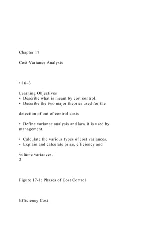
1. Chapter 17
Cost Variance Analysis
• 16–3
Learning Objectives
• Describe what is meant by cost control.
• Describe the two major theories used for the
detection of out of control costs.
• Define variance analysis and how it is used by
management.
• Calculate the various types of cost variances.
• Explain and calculate price, efficiency and
volume variances.
2
Figure 17-1: Phases of Cost Control
Efficiency Cost

2. • Total cost that results from an out of control
situation
• Efficiency Cost Equals
– T x R x P
– T = Total time from problem occurrence to
correction
– R = Loss or cost per time unit
– P = Probability that problem can be corrected
• 16–5
4
Alternatives for Minimizing
Efficiency Cost
• Preventive Approach
– Minimize P (Probability of a problem
occurring)
– Emphasis on right people with right motivation
• Detection-Correction Approach
– Minimize T (Total time problem is present)
– Emphasis on reporting and variance analysis
• 16–6
5

3. • 16–7
Variance Analysis
Requirements for variance analysis
• Standards (budgets)
• Related cost accounting system
• Fixed/variable split of costs
Phases in cost control
• Recognition of problem
• Determination of cause
• Correction
o Budgetary
o Operational
6
Alternative Methods to Determine
when to Investigate a Variance
• 16–8
• Control Chart
- Biggest problem is failure to
recognize costs of investigation
or benefits of problem correction
x = 0

4. x + 2σ
x - 2σ
7
Alternative Methods (cont.)
• Decision Theory (Payoff Table)
– I = Cost of Investigation
– L = Loss if system out of control
• 16–9
8
Alternative Methods (cont)
• Variances should be investigated if the
probability that the system is in control is less
than:
• Example –
– I = $1,000

5. – L = $4,000
– Investigate when probability of system being in
control is less than 75%
• 16–10
1.0 -
Cost of Investigation (I)
Loss if out of control (L)
9
Variance Analysis Areas
• Facility Level
– High level explanation of why costs have
changed
• Departments/Responsibility Centers
– Prior period cost analysis
– Budgetary cost comparisons
• Health Plan/Managed Care
• 16–11
10
• 16–12

6. Variance Analysis—Facility Level
Cost per discharge changes result from
• Resource price changes
• Productivity changes
• Intensity changes
Cost Equation
• CPD =
• Ci = Cost (charge) of service i
• Qi = Units of service i required per case
Ci * Qi
11
Σ
Variance Analysis – Facility
Level
• Two Indices split the variance into causes:
– HCI – change in cost due to price and
productivity
– HII – change in cost due to changes in service
intensity
• 16–13
12

7. Variance Analysis – Facility Level
• Change in cost per discharge
– CPD / CPD
– HCI x HII
• (HCI) is defined as the following:
• (HII) is defined as the following:
• 16–14
t
HCI =
C Q
C Q
t
0
0
0
HII =
C Q
C Q
t 0

8. 0 0
13
o
Variance Analysis – Facility Level
• Compute HCI
(C Q / C Q )
Variance Analysis – Facility Level
• Compute HCI
(C Q / C Q )
• 16–18
Variance Analysis – Summary
Total Cost / Discharge Example
2009 Cost / Discharge = $3,275.00
2011 Cost / Discharge = 4,310.34
% Increase 31.6%
HCI % 24.2%

9. HII % 5.5%
Joint % 1.9%
Total 31.6%
18
• 16–19
One Department (Lab)
HCI = = 1.143
HII = = 1.207
Variance Analysis (2009 to 2011)
Cost Increase % = 14.3
Intensity Increase % = 20.7
Joint Effect Increase % = 2.9
Total 37.9%
$85.71 x 5.0
$75.00 x 5.0
$75.00 x 6.0345
$75.00 x 5.0
Variance Analysis—Facility Level
19

10. Departmental Variance Analysis
• Causes of Variances
– Price (wages or prices of supplies differed from
budget)
– Efficiency (resource quantities used differed
from budget)
– Volume (actual volume of services differed
from budget)
– Utilization (output provided differed from what
was required)
• 16–20
20
• 16–21
Categories of Variances
Price
Efficiency
Volume
Variance = [Actual Price - Standard Price] x Actual Quantity

11. Variance = [Std. Volume - Actual Volume] x Avg. Fixed
Cost/Unit
Variance = [Actual Quantity - Std. Quantity] x Standard Price
Variance Analysis
Utilization
Variance = [Actual Volume – Expected Volume] x Standard
Cost per Unit
21
Table 17-8
Tabel 17-10
Department Variance Example
• Efficiency Variances
a) Head nurse = (180 – 189) x $30.00 = $270.00
(Favorable)
b) RN = (1,800 – 1,830) x $24.00 = $720.00
(Favorable)
c) LPN = (1,200-1,200) x $16.00 = 0
d) Aides = (2,400-2,430) x $10.00 = $300.00

12. (Favorable)
e) Supplies = (1,300 – 1,200) x $4.40 = $440.00
(Unfavorable)
• 16–25
25
Department Variance Example
• Price Variances
a) Head nurse = ($31.00-$30.00) x 180 = $180.00
(Unfavorable)
b) RN = ($25.00-$24.00) x 1,800 = $1,800.00 (Unfavorable)
c) LPN = ($16.20-$16.00) x 1,200 = $240.00 (Unfavorable)
d) Aides = ($9.60-$10.00) x 2,400 = $960.00 (Favorable)
e) Supplies = ($4.80-$4.40) x 1,300 = $520.00 (Unfavorable)
• Volume Variance
– Volume variance = (630 – 600) x $43.00 = $1,290.00
(Unfavorable)
• 16–26
26
Department Variance Example

13. • Utilization Variance
– Based on assumption that too much can be
included in an encounter of care, e.g. excessive
length of stay
– Assume in our example 80 cases with an
expected LOS of 7 days. We have excess days
of 40 (600-560)
– Utilization variance – (Act. Volume – Exp.
Volume) x Std. Cost per Unit
[600-560] x $161.80 = $6,472
• 16–27
27
Department Variance Analysis
• Summary
– Price Variance 1,780 (U)
– Efficiency Variance 850 (F)
– Volume Variance 1,290 (U)
– Utilization Variance 6,472 (U)
– Total 8,692 (U)
• 16–28
28
• 16–29

14. Variance Analysis Managed Care Contracts
• Cost = Inpatient (IP) + Outpatient (OP)
• IP = Admissions x Cost per Admission
= [Enrollees (E) x Admission per Member (APM)] x
[Cost per Admission (CPA) x Admission Case Mix Index
(ACMI)]
• OP = Visits x Cost Per Visit
= [Enrollees (E) x Visits per Member (VPM)] x
[Cost per Visit (CPV) x Visit Case Mix Index (VCMI)]
29
• Cost Drivers
1. Enrollment (E)
2. Utilization (APM or VPM)
3. Efficiency (CPA or CPV)
4. Patient Mix (ACMI or VCMI)
• Sample Data
• 16–30
Variance Analysis Managed Care Contracts

15. 30
Budget Actual
IP Costs $12,568,500 $16,531,200
OP Costs 5,433,120 5,372,640
Total 18,001,620 21,903,840
Members (E) 42,000 41,000
Admission Rate (APM) .070 .080
Admissions 2,940 3,280
Visit Rate (VPM) .400 .390
Visits 16,800 15,990
IP Case Mix (ACMI) .90 1.05
OP Case Mix (VCMI) 1.10 1.20
Cost per Admission (CPA) $4,750 $4,800
Cost per Visit (CPV) (VCMI = 1.0) $294 $280
• 16–31
• Enrollment Variance
= Change in Members x Budgeted Use Rates
x Budgeted Cost per Unit

16. 1. Inpatient
= (Ea - Eb) x APMb x CPAb x ACMIb
= -1000 x .07 x $4,750 x .90
= -$299,250 (Favorable)
2. Outpatient
= (Ea - Eb) x VPMb x CPVb x VCMIb
= -1000 x .400 x $294 x 1.10
= -$129,360 (Favorable)
Variance Analysis Managed Care Contracts
31
• 16–32
• Utilization Variances
= Change in Use Rates x Actual Members
x Budgeted Cost per Unit
1. Inpatient

17. = (APMa - APMb) x Ea x CPAb x ACMIb
= (.080 - .070) x 41,000 x $4,750 x .90
= $1,752,750 (Unfavorable)
2. Outpatient
= (VPMa - VPMb) x Ea x CPVb x VCMIb
= (.390 - .400) x 41,000 x $294 x 1.10
= -$132,594 (Favorable) 32
Variance Analysis Managed Care Contracts
• 16–33
• Efficiency
= Change in Cost per Unit x Actual Units
1. Inpatient
= (CPAa - CPAb) x ACMIa x Ea x APMa
= ($4,800 - $4,750) x 1.05 x 41,000 x .08
= $172,200 (Unfavorable)
2. Outpatient

18. = (CPVa - CPVb) x VCMIa x Ea x VPMa
= ($280 - $294) x 1.20 x 41,000 x .390
= -$268,632 (Favorable) 33
Variance Analysis Managed Care Contracts
• 16–34
• Patient Mix
= Change in Case Mix x Budget Cost per Unit
x Actual Volume
1. Inpatient
= (ACMIa - ACMIb) x CPAb x Ea x APMa
= (1.05 - .90) x $4,750 x 41,000 x .08
= $2,337,000 (Unfavorable)
2. Outpatient
= (VCMIa - VCMIb) x CPVb x Ea x VPMa
= (1.20 - 1.10) x $294 x 41,000 x .390
= $470,106 (Unfavorable) 34

19. Variance Analysis Managed Care Contracts
• 16–35
• Summary Variance Analysis (Negative Values are Favorable)
Enrollment
Utilization
Efficiency
Patient Mix
Total
($299,250)
1,752,750
172,200
2,337,000
$3,962,700
($129,360)

20. (132,594)
(268,632)
470,106
($60,480)
($428,610)
1,620,156
(96,432)
2,807,106
$3,902,220
Inpatient Outpatient Total
35
Variance Analysis Managed Care Contracts
Variance Analysis – Managed
Care

21. • Conclusions
– A large increase in both IP and OP case mix
increased costs
– IP usage was also up increasing costs
• 16–36
36
Chapter 17
Cost Variance Analysis
• 16–3
Learning Objectives
• Describe what is meant by cost control.
• Describe the two major theories used for the
detection of out of control costs.
• Define variance analysis and how it is used by
management.
• Calculate the various types of cost variances.
• Explain and calculate price, efficiency and

22. volume variances.
2
Figure 17-1: Phases of Cost Control
Efficiency Cost
• Total cost that results from an out of control
situation
• Efficiency Cost Equals
– T x R x P
– T = Total time from problem occurrence to
correction
– R = Loss or cost per time unit
– P = Probability that problem can be corrected
• 16–5
4
Alternatives for Minimizing
Efficiency Cost
• Preventive Approach
– Minimize P (Probability of a problem
occurring)
– Emphasis on right people with right motivation

23. • Detection-Correction Approach
– Minimize T (Total time problem is present)
– Emphasis on reporting and variance analysis
• 16–6
5
• 16–7
Variance Analysis
Requirements for variance analysis
• Standards (budgets)
• Related cost accounting system
• Fixed/variable split of costs
Phases in cost control
• Recognition of problem
• Determination of cause
• Correction
o Budgetary
o Operational
6
Alternative Methods to Determine
when to Investigate a Variance

24. • 16–8
• Control Chart
- Biggest problem is failure to
recognize costs of investigation
or benefits of problem correction
x = 0
x + 2σ
x - 2σ
7
Alternative Methods (cont.)
• Decision Theory (Payoff Table)
– I = Cost of Investigation
– L = Loss if system out of control
• 16–9
8
Alternative Methods (cont)

25. • Variances should be investigated if the
probability that the system is in control is less
than:
• Example –
– I = $1,000
– L = $4,000
– Investigate when probability of system being in
control is less than 75%
• 16–10
1.0 -
Cost of Investigation (I)
Loss if out of control (L)
9
Variance Analysis Areas
• Facility Level
– High level explanation of why costs have
changed
• Departments/Responsibility Centers
– Prior period cost analysis
– Budgetary cost comparisons

26. • Health Plan/Managed Care
• 16–11
10
• 16–12
Variance Analysis—Facility Level
Cost per discharge changes result from
• Resource price changes
• Productivity changes
• Intensity changes
Cost Equation
• CPD =
• Ci = Cost (charge) of service i
• Qi = Units of service i required per case
Ci * Qi
11
Σ
Variance Analysis – Facility
Level
• Two Indices split the variance into causes:
– HCI – change in cost due to price and

27. productivity
– HII – change in cost due to changes in service
intensity
• 16–13
12
Variance Analysis – Facility Level
• Change in cost per discharge
– CPD / CPD
– HCI x HII
• (HCI) is defined as the following:
• (HII) is defined as the following:
• 16–14
t
HCI =
C Q
C Q
t
0

28. 0
0
HII =
C Q
C Q
t 0
0 0
13
o
Variance Analysis – Facility Level
• Compute HCI
(C Q / C Q )
Variance Analysis – Facility Level
• Compute HCI
(C Q / C Q )
• 16–18

29. Variance Analysis – Summary
Total Cost / Discharge Example
2009 Cost / Discharge = $3,275.00
2011 Cost / Discharge = 4,310.34
% Increase 31.6%
HCI % 24.2%
HII % 5.5%
Joint % 1.9%
Total 31.6%
18
• 16–19
One Department (Lab)
HCI = = 1.143
HII = = 1.207
Variance Analysis (2009 to 2011)
Cost Increase % = 14.3
Intensity Increase % = 20.7
Joint Effect Increase % = 2.9
Total 37.9%
$85.71 x 5.0
$75.00 x 5.0

30. $75.00 x 6.0345
$75.00 x 5.0
Variance Analysis—Facility Level
19
Departmental Variance Analysis
• Causes of Variances
– Price (wages or prices of supplies differed from
budget)
– Efficiency (resource quantities used differed
from budget)
– Volume (actual volume of services differed
from budget)
– Utilization (output provided differed from what
was required)
• 16–20
20
• 16–21
Categories of Variances
Price

31. Efficiency
Volume
Variance = [Actual Price - Standard Price] x Actual Quantity
Variance = [Std. Volume - Actual Volume] x Avg. Fixed
Cost/Unit
Variance = [Actual Quantity - Std. Quantity] x Standard Price
Variance Analysis
Utilization
Variance = [Actual Volume – Expected Volume] x Standard
Cost per Unit
21
Table 17-8
Tabel 17-10
Department Variance Example

32. • Efficiency Variances
a) Head nurse = (180 – 189) x $30.00 = $270.00
(Favorable)
b) RN = (1,800 – 1,830) x $24.00 = $720.00
(Favorable)
c) LPN = (1,200-1,200) x $16.00 = 0
d) Aides = (2,400-2,430) x $10.00 = $300.00
(Favorable)
e) Supplies = (1,300 – 1,200) x $4.40 = $440.00
(Unfavorable)
• 16–25
25
Department Variance Example
• Price Variances
a) Head nurse = ($31.00-$30.00) x 180 = $180.00
(Unfavorable)
b) RN = ($25.00-$24.00) x 1,800 = $1,800.00 (Unfavorable)
c) LPN = ($16.20-$16.00) x 1,200 = $240.00 (Unfavorable)
d) Aides = ($9.60-$10.00) x 2,400 = $960.00 (Favorable)
e) Supplies = ($4.80-$4.40) x 1,300 = $520.00 (Unfavorable)
• Volume Variance

33. – Volume variance = (630 – 600) x $43.00 = $1,290.00
(Unfavorable)
• 16–26
26
Department Variance Example
• Utilization Variance
– Based on assumption that too much can be
included in an encounter of care, e.g. excessive
length of stay
– Assume in our example 80 cases with an
expected LOS of 7 days. We have excess days
of 40 (600-560)
– Utilization variance – (Act. Volume – Exp.
Volume) x Std. Cost per Unit
[600-560] x $161.80 = $6,472
• 16–27
27
Department Variance Analysis
• Summary
– Price Variance 1,780 (U)
– Efficiency Variance 850 (F)
– Volume Variance 1,290 (U)

34. – Utilization Variance 6,472 (U)
– Total 8,692 (U)
• 16–28
28
• 16–29
Variance Analysis Managed Care Contracts
• Cost = Inpatient (IP) + Outpatient (OP)
• IP = Admissions x Cost per Admission
= [Enrollees (E) x Admission per Member (APM)] x
[Cost per Admission (CPA) x Admission Case Mix Index
(ACMI)]
• OP = Visits x Cost Per Visit
= [Enrollees (E) x Visits per Member (VPM)] x
[Cost per Visit (CPV) x Visit Case Mix Index (VCMI)]
29
• Cost Drivers
1. Enrollment (E)

35. 2. Utilization (APM or VPM)
3. Efficiency (CPA or CPV)
4. Patient Mix (ACMI or VCMI)
• Sample Data
• 16–30
Variance Analysis Managed Care Contracts
30
Budget Actual
IP Costs $12,568,500 $16,531,200
OP Costs 5,433,120 5,372,640
Total 18,001,620 21,903,840
Members (E) 42,000 41,000
Admission Rate (APM) .070 .080
Admissions 2,940 3,280
Visit Rate (VPM) .400 .390
Visits 16,800 15,990
IP Case Mix (ACMI) .90 1.05
OP Case Mix (VCMI) 1.10 1.20
Cost per Admission (CPA) $4,750 $4,800

36. Cost per Visit (CPV) (VCMI = 1.0) $294 $280
• 16–31
• Enrollment Variance
= Change in Members x Budgeted Use Rates
x Budgeted Cost per Unit
1. Inpatient
= (Ea - Eb) x APMb x CPAb x ACMIb
= -1000 x .07 x $4,750 x .90
= -$299,250 (Favorable)
2. Outpatient
= (Ea - Eb) x VPMb x CPVb x VCMIb
= -1000 x .400 x $294 x 1.10
= -$129,360 (Favorable)
Variance Analysis Managed Care Contracts
31

37. • 16–32
• Utilization Variances
= Change in Use Rates x Actual Members
x Budgeted Cost per Unit
1. Inpatient
= (APMa - APMb) x Ea x CPAb x ACMIb
= (.080 - .070) x 41,000 x $4,750 x .90
= $1,752,750 (Unfavorable)
2. Outpatient
= (VPMa - VPMb) x Ea x CPVb x VCMIb
= (.390 - .400) x 41,000 x $294 x 1.10
= -$132,594 (Favorable) 32
Variance Analysis Managed Care Contracts
• 16–33
• Efficiency
= Change in Cost per Unit x Actual Units
1. Inpatient

38. = (CPAa - CPAb) x ACMIa x Ea x APMa
= ($4,800 - $4,750) x 1.05 x 41,000 x .08
= $172,200 (Unfavorable)
2. Outpatient
= (CPVa - CPVb) x VCMIa x Ea x VPMa
= ($280 - $294) x 1.20 x 41,000 x .390
= -$268,632 (Favorable) 33
Variance Analysis Managed Care Contracts
• 16–34
• Patient Mix
= Change in Case Mix x Budget Cost per Unit
x Actual Volume
1. Inpatient
= (ACMIa - ACMIb) x CPAb x Ea x APMa
= (1.05 - .90) x $4,750 x 41,000 x .08

39. = $2,337,000 (Unfavorable)
2. Outpatient
= (VCMIa - VCMIb) x CPVb x Ea x VPMa
= (1.20 - 1.10) x $294 x 41,000 x .390
= $470,106 (Unfavorable) 34
Variance Analysis Managed Care Contracts
• 16–35
• Summary Variance Analysis (Negative Values are Favorable)
Enrollment
Utilization
Efficiency
Patient Mix
Total
($299,250)
1,752,750

40. 172,200
2,337,000
$3,962,700
($129,360)
(132,594)
(268,632)
470,106
($60,480)
($428,610)
1,620,156
(96,432)
2,807,106
$3,902,220

41. Inpatient Outpatient Total
35
Variance Analysis Managed Care Contracts
Variance Analysis – Managed
Care
• Conclusions
– A large increase in both IP and OP case mix
increased costs
– IP usage was also up increasing costs
• 16–36
36