CONTROL

1. Chapter 5
PROCESS CONTROL

2. INTRODUCTION
 Control in process industries refers to the regulation of all
aspects of the process. Precise control of level, temperature,
pressure and flow is important in many process applications.
 This module introduces you to control in process industries,
explains why control is important, and identifies different
ways in which precise control is ensured.
 The following five sections are included in this module:
1. The importance of process control
2. Control theory basics
3. Components of Control Loops
4. Controller algorithms and tuning
5. Process control systems

3. 1) THE IMPORTANCE OF PROCESS CONTROL
The basic objectives of any process control system are:
1. Closely monitor the condition of the process
2. Maintain the process in a safe and stable condition
3. Compensate for changes in the process conditions and maintain
production to a given specification
4. Increase profitability
LEARNING OBJECTIVES
After completing this section, you will be able to:
 Define process
 Define process control
 Describe the importance of process control in terms of
variability, efficiency, and safety

4.  Process as used in the terms process control and process industry, refers to
the methods of changing or refining raw materials to create end products.
The raw materials, which either pass through or remain in a liquid, gaseous,
or slurry (a mix of solids and liquids) state during the process, are
transferred, measured, mixed, heated or cooled, filtered, stored, or handled
in some other way to produce the end product.
 Process industries include the chemical industry, the oil and gas industry, the
food and beverage industry, the pharmaceutical industry, the water treatment
industry, and the power industry.
 Process control refers to the methods that are used to control process
variables when manufacturing a product. For example, factors such as the
proportion of one ingredient to another, the temperature of the materials,
how well the ingredients are mixed, and the pressure under which the
materials are held can significantly impact the quality of an end product.

5.  Manufacturers control the production process for three reasons:
1. Reduce variability,
2. Increase efficiency,
3. Ensure safety
 Reduce Variability: Process control can reduce variability in the end
product, which ensures a consistently high-quality product. Manufacturers
can also save money by reducing variability. For example, in a gasoline
blending process, as many as 12 or more different components may be
blended to make a specific grade of gasoline. If the refinery does not have
precise control over the flow of the separate components, the gasoline may
get too much of the high-octane components. As a result, customers would
receive a higher grade and more expensive gasoline than they paid for, and
the refinery would lose money. The opposite situation would be customers
receiving a lower grade at a higher price.

6. Reducing variability can also save money by reducing the need for product
padding to meet required product specifications. Padding refers to the process
of making a product of higher-quality than it needs to be to meet specifications.
When there is variability in the end product (i.e., when process control is poor),
manufacturers are forced to pad the product to ensure that specifications are
met, which adds to the cost. With accurate, dependable process control, the
setpoint (desired or optimal point) can be moved closer to the actual product
specification and thus save the manufacturer money.

7. Increase Efficiency
 Some processes need to be maintained at a specific point
to maximize efficiency. For example, a control point might
be the temperature at which a chemical reaction takes
place. Accurate control of temperature ensures process
efficiency. Manufacturers save money by minimizing the
resources required to produce the end product.
Ensure Safety
 A run-away process, such as an out-of-control nuclear or
chemical reaction, may result if manufacturers do not
maintain precise control of all of the processing variables.
The consequences of a run-away process can be
catastrophic.
 Precise process control may also be required to ensure
safety. For example, maintaining proper boiler pressure by
controlling the inflow of air used in combustion and the
outflow of exhaust gases is crucial in preventing boiler
implosions that can clearly threaten the safety of workers.

8. 2) CONTROL THEORY BASICS
 This section presents some of the basic concepts of control and provides a foundation from
which to understand more complex control processes and algorithms later described in this
module. Common terms and concepts relating to process control are defined in this section.
 Learning Objectives
 After completing this section, you will be able to:
 Define control loop
 Describe the three tasks necessary for process control to occur:
» Measure
» Compare
» Adjust
 Define the following terms:
» Process variable
» Setpoint
» Manipulated variable
» Measured variable
» Error
» Offset
» Load disturbance
» Control algorithm
 List at least five process variables that are commonly controlled in process measurement
industries
 At a high level, differentiate the following types of control:
» Manual versus automatic feedback control
» Closed-loop versus open-loop control

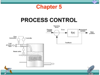
9. The Control Loop
 Control loops in the process control industry work in the same way, requiring three tasks to
occur:
» Measurement
» Comparison
» Adjustment
 In the figure, a level transmitter (LT) measures the level in the tank and transmits a signal
associated with the level reading to a controller (LIC). The controller compares the reading
to a predetermined value, in this case, the maximum tank level established by the plant
operator, and finds that the values are equal. The controller then sends a signal to the
device that can bring the tank level back to a lower level—a valve at the bottom of the tank.
The valve opens to let some liquid out of the tank.

10.  Summary of Control Terminology

11.  Process Variable: is a condition of the process fluid (a liquid or gas) that
can change the manufacturing process in some way.
 Setpoint: is a value for a process variable that is desired to be
maintained. For example, if a process temperature needs to kept within
5°C of 100°C, then the setpoint is 100°C. A temperature sensor can be
used to help maintain the temperature at setpoint.
 Measured variable is the condition of the process fluid that must be kept
at the designated setpoint. Sometimes the measured variable is not the
same as the process variable. For example, a manufacturer may
measure flow into and out of a storage tank to determine tank level. In
this scenario, flow is the measured variable, and the process fluid level is
the process variable. The factor that is changed to keep the measured
variable at setpoint is called the manipulated variable.

12. Types of thermocouples
 Error is the difference between the measured variable and the setpoint
and can be either positive or negative. The objective of any control scheme
is to minimize or eliminate error. Therefore, it is imperative that error be well
understood.
 Magnitude of the error is simply the deviation between the values of the
setpoint and the process variable. The magnitude of error at any point in time
compared to the previous error provides the basis for determining the change
in error. The change in error is also an important value.
 Duration refers to the length of time that an error condition has existed.
 Rate of Change is shown by the slope of the error plot.

13.  Offset is a sustained deviation of the process variable from the setpoint. In the
temperature control loop example, if the control system held the process fluid at
100.5°C consistently, even though the setpoint is 100°C, then an offset of 0.5°C
exists.
 Load Disturbance: is an undesired change in one of the factors that can affect
the process variable. In the temperature control loop example, adding cold
process fluid to the vessel would be a load disturbance because it would lower
the temperature of the process fluid.
 Control Algorithm: is a mathematical expression of a control function. Using the
temperature control loop example, V in the equation below is the fuel valve
position, and e is the error. The relationship in a control algorithm can be
expressed as:
 The fuel valve position (V) is a function (f) of the sign (positive or negative) of the
error.

14. Manual and Automatic Control
 Before process automation, people, rather than machines, performed many of
the process control tasks. For example, a human operator might have watched
a level gauge and closed a valve when the level reached the setpoint. Control
operations that involve human action to make an adjustment are called
manual control systems.

15.  Conversely, control operations in which no human intervention is required, such as an
automatic valve actuator that responds to a level controller, are called automatic control
systems.
 Automatic control systems produce:
• A more consistent product
• Release skilled operators for other productive work
• Reduce the physical effort required, lessening fatigue and boredom
• Decrease the physical workload on an operator
• Improve safety and working conditions
 Once an automatic control system has been installed and commissioned, it should be
able to maintain a pre-set operating condition over an extended period of time without
any operator involvement.

16. Open and Closed Control Loops
 An open control loop exists where the process variable is not
compared, and action is taken not in response to feedback on the
condition of the process variable, but is instead taken without regard
to process variable conditions.
 Open loop control has no information or feedback about the measured
value.
 The position of the correcting element is fixed.
 It is unable to compensate for any disturbances in the process.

17.  A closed control loop exists where a process variable is measured, compared to
a setpoint, and action is taken to correct any deviation from setpoint.
 In a closed loop control system the output of the measuring element is fed into the
loop controller where it is compared with the set point. An error signal is generated
when the measured value is not equal to the set point. Subsequently, the
controller adjusts the position of the control valve until the measured value fed into
the controller is equal to the set point.
 Closed loop control has information and feedback about the measured value.
 The position of the correcting element is variable.
 It is able to compensate for any disturbances in the process.

18. 3) COMPONENTS OF CONTROL LOOPS
 This section describes the instruments, technologies, and equipment
used to develop and maintain process control loops.
Control Loop Equipment and Technology
 The basic elements of control as measurement, comparison, and
adjustment. In practice, there are instruments and strategies to
accomplish each of these essential tasks.

19.  Primary elements are devices that cause some change in their property with
changes in process fluid conditions that can then be measured.
 Transducer is a device that translates a mechanical signal into an electrical
signal. For example, inside a capacitance pressure device, a transducer converts
changes in pressure into a proportional change in capacitance.
 Converter is a device that converts one type of signal into another type of signal.
 Transmitter is a device that converts a reading from a sensor or transducer into a
standard signal and transmits that signal to a monitor or controller
 Signals: There are three kinds of signals that exist for the process industry to
transmit the process variable measurement from the instrument to a centralized
control system.
1. Pneumatic signal: are signals produced by changing the air pressure in a signal pipe in
proportion to the measured change in a process variable. The common industry
standard pneumatic signal range is 3–15 psig.
2. Analog signal: The most common standard electrical signal is the 4–20 mA current
signal. With this signal, a transmitter sends a small current through a set of wires.
3. Digital signal: are discrete levels or values that are combined in specific ways to
represent process variables and also carry other information, such as diagnostic
information. The methodology used to combine the digital signals is referred to as
protocol.

20.  Indicator is a human-readable device that displays information about the
process.
 Recorder is a device that records the output of a measurement devices.
 Chart recorders: Recorders that create charts or graphs.
 Controller is a device that receives data from a measurement instrument,
compares that data to a programmed setpoint, and, if necessary, signals a
control element to take corrective action.
» controllers are usually one of the three types: pneumatic, electronic or
programmable. Controllers also commonlyreside in a digital control system.
 Correcting or final control element is the part of the control system that
acts to physically change the manipulated variable.
 Actuator is the part of a final control device that causes a physical change
in the final control device when signalled to do so.

21. 4) CONTROLLER ALGORITHMS AND TUNING
After completing this section, you will be able to:
 Differentiate between discrete, multistep, and continuous controllers
 Describe the general goal of controller tuning.
 Describe the basic mechanism, advantages and disadvantages of the
following mode of controller action:
» Proportional action
» Integral action
» Derivative action
 Give examples of typical applications or situations in which each mode of
controller action would be used.
 Identify the basic implementation of P, PI and PID control in the following
types of loops:
» Pressure loop
» Flow loop
» Level loop
» Temperature loop

22. Controller Algorithms
 The actions of controllers can be divided into
groups based upon the functions of their control
mechanism. Each type of controller has
advantages and disadvantages and will meet the
needs of different applications. Grouped by control
mechanism function, the three types of controllers
are:
» Discrete controllers
» Multistep controllers
» Continuous controllers

23.  Discrete controllers are controllers that have only two modes or
positions: on and off (two-step). This type of control doesn’t actually hold
the variable at setpoint, but keeps the variable within proximity of setpoint
in what is known as a dead zone.
 Two-step is the simplest of all the control modes. The output from the
controller is either on or off with the controller's output changing from one
extreme to the other regardlessof the size of the error.

24. Advantages of ON-OFF Control:
 On/Off control makes "trouble shooting" very easy and requires only
basic types of instruments.
Disadvantages of ON-OFF Control:
 The process oscillates.
 The final control element (usually a control valve) is always opening
and closing. This causes excessive wear.
 There is no fixed operating point.

25.  Multistep controllers are controllers that have at least one other
possible position in addition to on and off. Multistep controllers operate
similarly to discrete controllers, but as setpoint is approached, the
multistep controller takes intermediate steps. Therefore, the oscillation
around setpoint can be less dramatic when multistep controllers are
employed than when discrete controllers are used.

26. Continuous Controllers
 Controllers automaticallycompare the value of the PV to the SP to determine if
an error exists. If there is an error, the controller adjusts its output according to
the parameters that have been set in the controller. The tuning parameters
essentially determine:
» How much correction should be made? The magnitude of the correction (change in
controller output) is determined by the proportional mode of the controller.
» How long the correction should be applied? The duration of the adjustment to the
controller output is determined by the integral mode of the controller
» How fast should the correction be applied? The speed at which a correction is made is
determined by the derivative mode of the controller.

27. Proportional Action
 With proportional control action, the correcting element is adjusted In proportion to
the change in the measured value from the set point. The largest movement is made
to the correcting element when the deviation between measured value and set point
is greatest. Usually, the set point and measured value are equal when the output is
midway of the controller output signal range.
 In the accompanying diagram, the set point is shown at 60%, the measured value at
75% and the output at 65%. If the measured value were to drop to 60%, that is, equal
to the SP, the output would stabilise at the designed 50%. By repositioning the set
point to 50% the measured value falls to 50%, the output would again be 50%.
 Assuming that the level transmitter, controller and control valve are all operating
correctly and have been recently calibrated, when set point and measured value are
equal and the system is in stable condition, the valve will be 50% open. The valve
would have been sized during design to maintain the stable condition under a set of
known conditions.

28.  The process throughput, the fluid condition, the vessel, operating
pressure and the back-pressure from the downstream process can all
affect the throughput of the control valve. From .the diagram, it can be
seen that the process input is equal to the process output and steady
state conditions have been achieved with a level stabilised at 75%, but
with a SP of 60%.
 Under these conditions, the control valve would need to be 65% open;
the magnitude of deviation is used to reposition the valve from its normal
50% open position. Deviation from other changes in operating
conditions, particularly load changes, would also open or close the valve
to achieve the new stable level.

29.  The process load can be changed in the following ways to
remove the deviation:
» Reduce the process input to the vessel allowing the level to drop so
that a stable level is achieved at 60%'when the valve is 50% open.
» Increase the operating pressure of the vessel. This creates a higher
differential pressure across the control valve, causing the fluid to
flow from the vessel at an increased rate. This allows the level to'
fall so that» a stable level is achieved at 60% when the valve is
50% open.
» Reduce the back pressure from the downstream process, creating
a higher differential pressure across the control valve. This also
causes the fluid to flow from the vessel at an increased rate.
» Increase the capacity of the control valve to allow more process
fluid to flow through the valve so that at 50% open a 60% level in
the vessel is achieved.
» Any combination of the above conditions will also remove the
deviation. Over compensation may cause the measured value to
move below the set point, causing a deviation in the opposite
direction.

30. Proportional Mode:
 The simplest and most common form of control action to be found on a
controller is proportional. With this form of control the output from the
controller is directly proportional to the input error signal, i.e. the larger
the input error the larger the output response from the controller.
 The actual size of the output depends on another factor, the controller's
proportional band or gain. (The controller's sensitivity)
 The setting for the proportional mode may be expressed as either:
» Proportional Band (PB) is another way of representing the same
information and answers this question: "What percentage of change
of the controller input span will cause a 100% change in controller
output?“ PB = Δ Input (% Span) For 100%Δ Output.
» Proportional Gain (Kc) answers the question: "What is the percentage
change of the controller output relative to the percentage change in
controller input?“ Proportional Gain is expressed as: Gain, (Kc) = Δ
Output% / Δ Input %

31. Converting Between PB and Gain
 Gain is just the inverse of PB multiplied by 100 or gain = 100/PB
 PB = 100/Gain
 Also recall that: Gain = 100% / PB
 Proportional Gain, (Kc) = Δ Output% / Δ Input %
 PB= Δ Input (%Span) For 100% Δ Output

32.  The proportional mode of control can be described mathematically as:
V = K (E) + M
Where
» V = controller output signal to correcting unit,
» K = adjustable gain,
» E = magnitude of error signal,
» M = constant which is the position of the valve when there is no deviation,
that is, SP = MV and E = 0.
 This can be shown diagrammatically as in the following diagram and
gain settings can be shown graphically as in the following diagram.

33. Summary of Proportional control
With Proportional Control:
» Δ Controller Output = (Change in Error)(Gain)
» Proportional Mode Responds only to a change in error
» Proportional mode alone will not return the PV to SP.
» Stable control
» Suffers from offset due to load changes.
 Narrow PB%
» Fast to respond,
» Large overshoot,
» Long settling time,
» Small offset
 Wide PB%
» Slow to respond,
» Quick to settle’
» Large offset
 Proportional control used in process where load changes are small and the offset can be tolerated.
 Tuning - reduce PB (increase gain) until the process cycles following a disturbance, then double the PB (reduce gain by
50%).
 With Optimum Setting of P Control

34. Integral Mode
Integral Action
 Another component of error is the duration of the
error, i.e., how long has the error existed?. The
controller output from the integral or reset mode is a
function of the duration of the error.
 Integral action is used in conjunction with
proportional action to eliminate offset problem
resulting from P control.
 This is accomplished by repeating the action of the
proportional mode as long as an error exists.

35.  An example of integral action in P + I controller is shown in the following diagram, here if
the process is operating under steady state conditions at a set point of, say, 40% at time T
= 0 minutes, the output of the controller is at 20%. In a proportional only controller the
output would be 50% when the measured value is equal to set point, but this is not
necessarily the case In a proportional plus reset controller.
 At the time T = 0.2 minutes a sudden load change occurs which causes the measured
value to rise 20% above set point to 60%. Proportional action increases the output 20% to
40%, which indicates a PB of 100% or a gain of 1.
 If the offset is maintained after this output change because the increased output cannot
cause the measured variable to drop, the controller output will begin to increase in a ramp
fashion.
 The time it takes to ramp the controller output up to a value equal to the effect of the initial
proportional action is called the integral action time. So the initial proportional action is a
20% increase in output. This action is repeated by integral action in 0.4 - 0.2 = 0.2 minutes
to move the output from 40% to 60%, so for this example, integral action time = 0.2
minutes per repeat = 5 repeats/min.

36.  Integral Action Effect

37. Integral Saturation or Reset Wind-up
 A common problem caused by integral action is called integral saturation
or wind-up. During the time a process is shut down the integral action will
keep trying to move the valve to correct for the error between its set point
and the actual process value. When the process is started up it will take
time for the process controller to gain control of the valve again. This time
delay could result in damage to the plant or shutdown due to the plant
safety devices cutting in. Normally a process such as this would be
brought up on manual control and then switched over to automatic.
 To prevent saturation from occurring controllers are fitted with integral de-
saturation or anti wind-up devices. De-saturation relays prevent the
controller's output from falling below 3 psi and rising above 1 psi.

38. Summary of integral action (Reset)
 Integral (Reset) Summary - Output is a repeat of the proportional action as long as error exists. The
units are in terms of repeats per minute or minutes per repeat.
 Advantages - Eliminates error
 Disadvantages: Makes the process less stable and take longer to settle down.
 Can suffer from integral saturation or wind-up on batch processes.
 Fast Reset (Large Repeats/Min., Small Min./Repeat)
» High Gain
» Fast Return To Setpoint
» Possible Cycling
 Slow Reset (Small Repeats/Min., Large Min./Repeats)
» Low Gain
» Slow Return To Setpoint
» Stable Loop
 P + I controller is used when offset must be eliminated automatically and integral saturation due to a
sustained offset is not a problem.
 Trailing and Error Tuning - Increase repeats per minute until the PV cycles following a disturbance,
then slow the reset action to a value that is 1/3 of the initial setting.

39. Derivative Mode
Why Derivative Mode?
 Some large and/or slow process do not respond well to small changes in controller output. For
example, a large liquid level process or a large thermal process (a heat exchanger) may react
very slowly to a small change in controller output. To improve response, a large initial change in
controller output may be applied. This action is the role of the derivative mode.
 The derivative action is initiated whenever there is a change in the rate of change of the error
(the slope of the PV). The magnitude of the derivative action is determined by the setting of the
derivative.
 In operation, the controller first compares the current PV with the last value of the PV. If there is
a change in the slope of the PV, the controller determines what its output would be at a future
point in time (the future point in time is determined by the value of the derivative setting, in
minutes). The derivative mode immediately increases the output by that amount.

40.  Derivative Action:
 The following illustration shows the effect of derivative action when a constant rate of
change of offset is considered [the derivative time is 0.4 minutes (1 - 0.6)]. When the set
point is equal to the measured value the output remains constant.
 Once the rate at which the measured value is increasing from the set point is
determined, then derivative action acts to increase the controller output, in this case,
from 30% to 50%. The output then increases due to proportional action.
 The additional correction exists only while the error is changing, it disappears when the
error stops changing even-though there may still be a large value of error signal.
 Derivative action has no effect on the offset in a proportional only controller and therefore
it is unusual to find a proportional plus derivative controller.

41. Summary of Derivative action (Rate)
 Rate action is a function of the speed of change of the error. The units are minutes. The action is to
apply an immediate response that is equal to the proportional plus reset action that would have occurred
some number of minutes I the future.
 Advantages - Rapid output reduces the time that is required to return PV to SP in slow process.
 Disadvantage - Has no effecton offset. Dramatically amplifies noisy signals; can cause cycling in fast
processes.
 Large (Minutes):
» High Gain
» Large Output Change
» Possible Cycling
 Small (Minutes):
» Low Gain
» Small Output Change
» Stable Loop
 Trial-and-Error Tuning
» Increase the rate setting until the process cycles following a disturbance, then reduce the rate setting to one-third of
the initial value.

42. Proportional, PI, and PID Control
 By using all three control algorithms together, process operators can:
» Achieve rapid response to major disturbances with derivative control
» Hold the process near setpoint without major fluctuations with proportional control
» Eliminate offset with integral control
 Not every process requires a full PID control strategy. If a small offset has no
impact on the process, then proportional control alone may be sufficient.
 PI control is used where no offset can be tolerated, where noise (temporary error
readings that do not reflect the true process variable condition) may be present,
and where excessive dead time (time after a disturbance before control action
takes place) is not a problem.
 In processes where no offset can be tolerated, no noise is present, and where
dead time is an issue, customers can use full PID control.

43.  Summary of Control modes and responses

44. Automatic Controller Adjustments
 Set point adjustment, which allows the operator to select the required operating
point for the process when the controller is in automatic mode.
 Auto/manual selector switch. When in the manual position the controller output
becomes independent of the measured value and set point, that is, the
controller 'operates in open loop.
 Output adjustment which allows the position of the final control element to be
controlled by the operator when the controller is in manual mode so that the
correcting element can be moved from fully closed to fully open and can be
held at any position in between.

45. Bumpless Transfer
 When switching a controller from auto to manual or vice versa, care must be
taken that the output signal does not move sharply when the auto/manual
switch is operated. This may cause a severe disturbance in the process, which
may result in damage or shutdown.
 Switch Auto to Manual
» Adjust manual output until the balance indicator shows that the manually adjusted
output pressure is equal to the output pressure generated by the auto mechanism.
The balance indicator mechanism varies according to the manufacturer of the
controller, but all indicate by a flag or some similar device when the two output
pressures are equal.
» Once the balance position has been found, It Is safe to switch from auto to manual
without any process bump. The manual output adjustment now has control of the
output to the final control element.
 Switch Manual to Auto
» When switching from manual to auto, the set point should Initially be moved towards
the measured value to see if an output balance can be found. It is usual to find
balance where there is an offset between set point and measured value. When the
balance point has been found, it is then safe to switch to auto and slowly reposition
the set point to the desired operating condition.

46. Controller Tuning
Why Controllers Need Tuning?
 Controllers are tuned in an effort to match the characteristics of the control
equipment to the process so that two goals are achieved; is the foundation of
process control measurement in that electricity:
» The system responds quickly to errors.
» The system remains stable (PV does not oscillate around the SP)
 Controller tuning is performed to adjust the manner in which a control valve (or
other final control element) responds to a change in error.
 In particular, we are interested in adjusting the controller’s modes (gain, Integral
and derivative), such that a change in controller input will result in a change in
controller output that will, in turn, cause sufficient change in valve position to
eliminate error, but not so great a change as to cause instability or cycling.
 There are many trial and error methods of controller tuning which do not involve
mathematical analysis and should be demonstrated by an experienced person,
otherwise shutdowns may occur.
 The first adjustment, which would normally be made, would be to set forward or
reverse action as required. A forward acting controller has increasing output in
response to an increasing measured variable. A reverse acting controller has
decreasing output in response to an increasing measured variable.

47.  PB at Optimum Value
 Controller optimisations can then be carried out as follows. For any
particular control system there is a value of the proportional band, which
will produce the best controller performance:
» Increasing the proportional band above this value will result in greater
deviations of the controlled condition from the desired value owing to
disturbances in the process.
» Decreasing the Proportional band below the critical value will
increase the tendency for the process to hunt, and disturbances will
cause prolonged oscillation of the controlled condition about the
control point. Indeed, if made too narrow, the system becomes
unstable and instead of the oscillations dying out they will increase in
amplitude.
 Trained observation of the chart record, following a plant disturbance,
thus provides a method of initially adjusting a controller's settings to the
process. Process disturbances are easily simulated by moving the set
point away from the desired value and returning it to its original position.

48. Empirical Tuning Method
 Proportional only controller
» With transfer switch at manua1, set PB at maximum or at safe high value,
usually 200% PB.
» Move transfer switch to auto and make changes in set point. The time
required for the disturbance to settle may then be noted.
» Continue reducing band-width to half its previous value until the oscillation do
not die away, But continue to be perceptible.
» Now increase the band-width to twice its value. This gives the required
stability, that is, the minimum stabilising time and minimum offset.
 Proportional plus integral action
» Set the Integral Action Time (IAT) to maximum.
» Adjust the proportional band as for a proportional controller.
» Decrease the IAT in steps, each step being such that line IAT 1s halved at
each adjustment. Below some critical value, depending upon the lag
characteristics of the process, hunting will occur. This hunting Indicates that
the IAT has been reduced too far.
» Now increase the time to approximately twice this value to restore the desired
stability.

49.  Proportional plus derivative action
» Adjust the Derivative Action Time (DAT) to its minimum value.
» Adjust the proportional band as described for proportional
controller, but do not increase the band when hunting occurs.
» Increase the DAT (that is, double each setting) so that; the hunting
caused by the narrow band is eliminated.
» Continue to narrow the band and again increase the DAT until the
hunting is eliminated.
» Repeat previous step until further increase of the derivative action
time fails to eliminate the hunting introduced by the reduction of the
proportional band, or tends to increase it. This establishes the
optimum value of the DAT and the hunting should be eliminated by
increasing the width of the proportional band slightly.
 Proportional plus integral plus derivative action
» Set IAT to a maximum.
» Set DAT to a minimum.
» Adjust the proportional band as for a P + D controller.
» Adjust derivative using same procedure as for above, P + D.
» Adjust integral to a related value of the final derivative setting.

50.  In many cases, the setting procedure may be shortened by omitting
settings, which are outside the probable range.
 The process should then respond to set point or load changes, where
integral action removes offset and the second overshoot of set point is
approximately 1/4 the amplitude of the first. This is commonly referred to
as the 1/4 decay method and is generally agreed to be the optimum
controller setting for a P + I controller.
 The above method is only used when no other controller setting data is
available and must be practised with care.

51. Optimum Settings (Ultimate Method)
 The closed loop or ultimate method involves finding the point where
the system becomes unstable and using this as a basis to calculate
the optimum settings.
 The following steps may be used to determine ultimate PB and period:
1. Switch the controller to Manual and set the proportional band to high
value.
2. Turn off all integral and derivative action.
3. Switch the controller to automatic and reduce the proportional band value
to the point where the system becomes unstable and oscillateswith
constant amplitude. Sometimes a small step change is required to force
the system into its unstable mode. The below figure showing typical
response obtained when determining ultimate proportional band and
ultimate period time.
4. The proportional band that required causing continuous oscillation is the
ultimate value Bu.
5. The ultimate periodic time is Pu.
6. From these two values the optimum setting can be calculated as per the
following procedures.

52.  Look for curve B that represents the continuous oscillation

53. Optimum setting calculation
 For proportional action only
» PB% = 2 Bu %
 Proportional + Integral
» PB% = 2.2 Bu %
» Integral action time = Pu / 1.2 minutes/repeat
 Proportional + Integral + Derivative
» PB%=1.67Bu
» Integral action time = Pu / 2 minutes/repeat
» Derivative action = Pu / 8 minutes

55. 5) PROCESS CONTROL LOOPS
 In this section, you will learn about how control components and control algorithms are integrated to create a
process control system. Because in some processes many variables must be controlled, and each variable
can have an impact on the entire system, control systems must be designed to respond to disturbances at
any point in the system and to mitigate the effect of those disturbances throughout the system.
Learning Objectives:
After completing this section, you will be able to:
 Explain how a multivariable loop is different from a single loop.
 Differentiate feedback and feedforward control loops in terms of their operation, design, benefits, and
limitations
 Perform the following functions for each type of standard process control loop (i.e., pressure, flow, level, and
temperature):
» State the type of control typically used and explain why it is used
» Identify and describe considerations for equipment selection (e.g., speed, noise)
» Identify typical equipment requirements
 Explain the basic implementation process, including a description of equipment requirements and
considerations, for each of the following types of control:
» Cascade control
» Ratio control
» Override control
» End-point control
» Batch control
» Fuzzy control
 Describe benefits and limitations of each type of control listed above
 Give examples of process applications in which each type of control described in this section might be used

56. 5.1) Single Control Loops
 Feedback Control loop: measures a process variable and sends the
measurement to a controller for comparison to setpoint. If the process variable is
not at setpoint, control action is taken to return the process variable to setpoint. In
the figure, a feedback loop in which a transmitter measures the temperature of a
fluid and, if necessary, opens or closes a hot steam valve to adjust the fluid’s
temperature.
 Feedback loops are commonlyused in the process control industry. The
advantage of a feedback loop is that it directly controls the desired process
variable. The disadvantage to feedback loops is that the process variable must
leave setpoint for action to be taken.

57. Examples of feedback Control Loops

58.  Feedforward control is a control system that anticipates load disturbances and
controls them before they can impact the process variable. For feedforward
control to work, the user must have a mathematicalunderstanding of how the
manipulated variables will impact the process variable. In the figure the flow
transmitter opens or closes a hot steam valve based on how much cold fluid
passes through the flow sensor.
 An advantage of feedforward control is that error is prevented, rather than
corrected. However, it is difficult to account for all possible load disturbances in a
system through feedforward control. Factors such as outside temperature,
buildup in pipes, consistencyof raw materials, humidity, and moisture content can
all become load disturbances and cannot always be effectively accounted for in a
feedforward system.

59. 5.2) Multi-Variable / Advanced Control Loops
 Multivariable loops are control loops in which a primary
controller controls one process variable by sending signals
to a controller of a different loop that impacts the process
variable of the primary loop.
 When tuning a control loop, it is important to take into
account the presence of multivariable loops. The standard
procedure is to tune the secondary loop before tuning the
primary loop because adjustments to the secondary loop
impact the primary loop. Tuning the primary loop will not
impact the secondary loop tuning.

60. Feedforward Plus Feedback
 Because of the difficultyof accounting for every possible load disturbance in a
feedforward system, feedforward systems are often combined with feedback
systems. Controllers with summing functions are used in these combined systems
to total the input from both the feedforward loop and the feedback loop, and send a
unified signal to the final control element.
 In the figure a feedforward-plus-feedback loop in which both a flow transmitter and
a temperature transmitter provide information for controlling a hot steam valve.

61. Cascade Control
 Cascade control is a technique that uses two
measuring and control systems to manipulate a
single final control element. Its purpose is to provide
increased stability to particularly complex process
control problems. The technique has been used for
many years and is very effective in many
applications.
 Cascade control accomplishes two important
functions:
» it reduces the effect of load changes near their source,
and
» it improves control by reducing the effect of time lags.

62.  The schematic shows how control is accomplished directly
with the temperature controller regulating steam flow
through the heating coil. This system works very well
except when disturbances occur in the feed rate or when
steam pressure variations change the amount of flow
through the heating coil. Because of the fluid capacity in
the vessel and because of the measurement lag time, the
temperature controller does not immediately detect the
disturbances. By the time detection is made, the
disturbance may have receded to its normal operation.
Cyclic action probably occurs.

63.  IN this schematic, illustrates how the cascade system operates. The
steam feed is placed on now control so that the desired steam now is
maintained despite pressure fluctuations in the supply. The
temperature controller is cascaded with the flow controller, however, so
that long-range fluctuations such as feed rate, ambient temperature
effects, etc., will be overcome, and the desired variable (temperature)
is maintained as needed. It resets the flow control set point as
necessary to maintain the correct temperature.
 Cascade systems can be overemphasized; they are not a panacea for
every unstable process condition encountered or for all measurement
lag problems. However, they do provide satisfactory solutions to many
application problems.

64. Ratio Control
 As the name implies, ratio control is maintaining a fixed ratio between
two variables. The most common application for ratio control is
maintaining a fixed relationship between two flows, such as air-fuel ratios
in furnaces, feed and catalysts ratios in reactors and mixtures of two or
more raw materials in blending operation.
 In this figure: The uncontrolled flow (A) is measured and an adjustable
ratio linkage on the controller is used to control flow (B) to the desired
ratio between A and B.

65.  A more common method of ratio control is using separate
units to provide the ratio system. In this figure, the
measurement of an uncontrolled flow transmitted to a ratio
unit where it is multiplied by a ratio factor, and the output of
the ratio unit becomes the set point of the secondary
controller. The ratio unit normally has a manually adjusted
scale to adjust the ratio between the two variables.

66. Override Control
 In process control systems it often becomes desirable to
limit a process variable to some low or high value to avoid
damage to process equipment or to the product. This is
accomplished by override devices. As long as the variable is
within the limits set by the override devices, normal
functioning of the control system continues; when the set
limits are exceeded, the override devices take
predetermined actions.

67. Time-Cycle Control
 Time-cycle control involves one or more circuits, usually
electrical, which activate on-off valves and other control
devices to perform repetitive operations in process
operations.
 There are many process functions that require this type
control for entire operational sequences. Some functions
are simple, such as switching drying chambers in dessicant
air dryers that have two dessicant beds used alternately in
the drying and reactivation cycles.
 Other more complex systems include absorbent type drying
systems such as molecular sieves for moisture removal or
other liquid or component separation. Such systems as
these involve switching, furnace operation and other on-off
functions that are accomplished on a pure time cycle or a
combination of time cycle and end-point control.

68. End-Point Control
 End-point control is a combination of control systems in which a primary variable automatically adjusts
set points or ratios of controllers to achieve control of the primary variable.
 In the example a process must be neutral at the mixing tank to prevent unnecessary corrosion to
process equipment downstream. A combination of cascade and ratio unit control systems is used for
this purpose.
 End-point analysis is made by a pH detector, and its controller adjusts the ratio of the neutralizing
agent (secondary flow) to the acid stream (primary flow) to achieve a neutralized (basic) mixture. As
acidity changes in the primary stream, the pH controller detects the deviation from set point and
adjusts the ratio setting automatically to keep the mixture under control.
 This technique can also be applied to controlling air-fuel ratio in furnaces by measuring the oxygen
content of the exhaust gases.

69. Batch Control (Program Control)
 Batch processes are those processes that are taken from
start to finish in batches. For example, mixing the
ingredients for a juice drinks is often a batch process.
Typically, a limited amount of one flavor (e.g., orange drink
or apple drink) is mixed at a time. For these reasons, it is
not practical to have a continuous process running. Batch
processes often involve getting the correct proportion of
ingredients into the batch. Level, flow, pressure,
temperature, and often mass measurements are used at
various stages of batch processes.
 A disadvantage of batch control is that the process must be
frequently restarted. Start-up presents control problems
because, typically, all measurements in the system are
below setpoint at start-up. Another disadvantage is that as
recipes change, control instruments may need to be
recalibrated.

70. Fuzzy Control
 Fuzzy control is a form of adaptive control in which the
controller uses fuzzy logic to make decisions about
adjusting the process. Fuzzy logic is a form of computer
logic where whether something is or is not included in a set
is based on a grading scale in which multiple factors are
accounted for and rated by the computer. The essential idea
of fuzzy control is to create a kind of artificial intelligence
that will account for numerous variables, formulate a theory
of how to make improvements, adjust the process, and
learn from the result.
 Fuzzy control is a relatively new technology. Because a
machine makes process control changes without consulting
humans, fuzzy control removes from operators some of the
ability, but none of the responsibility, to control a process.