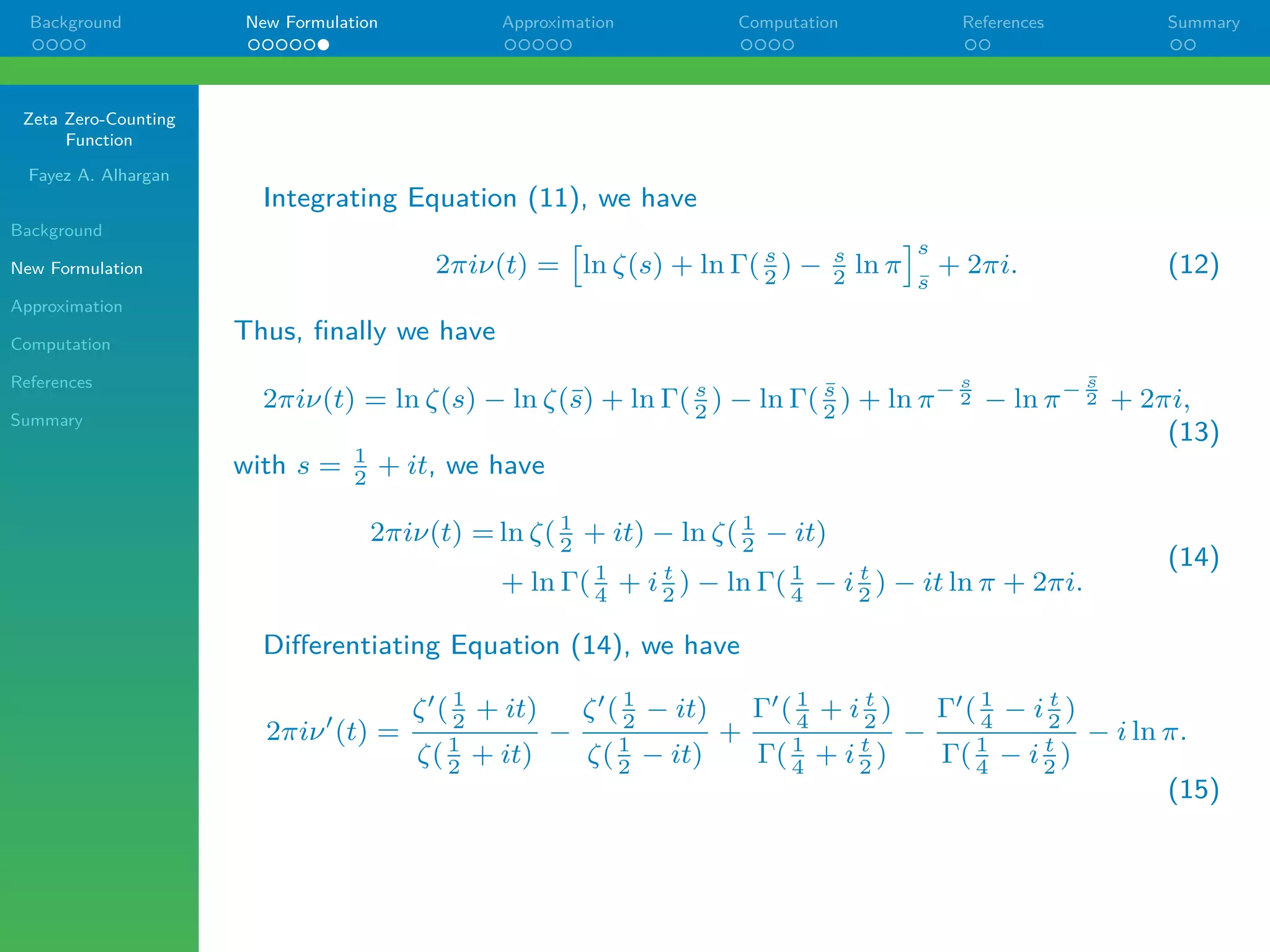
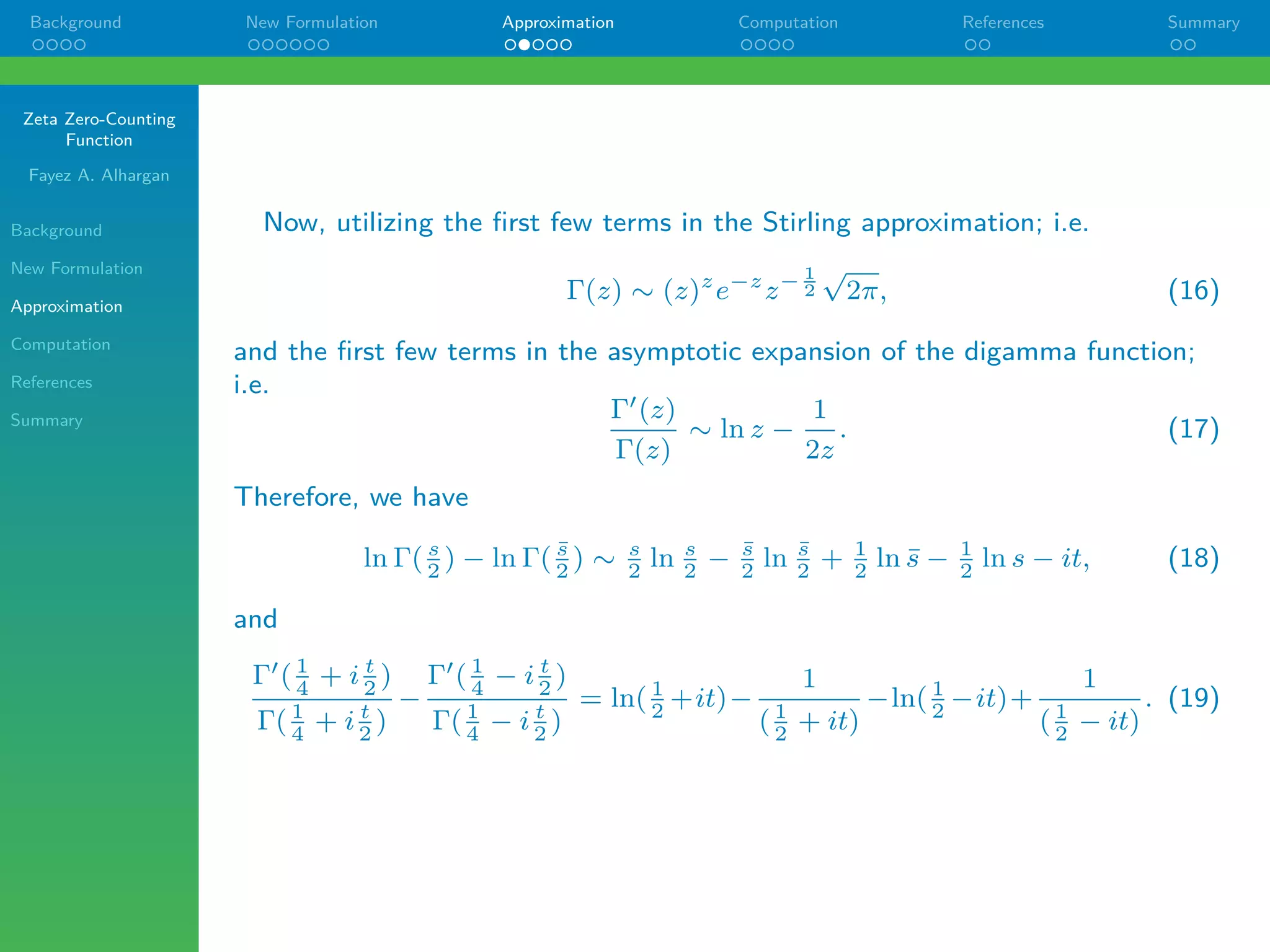
The document presents a new formulation for the zeta zero-counting function, improving upon prior approximations established by Riemann and von Mangoldt. It develops a more accurate expression demonstrating the relationship between the zeta zeros and prime numbers, highlighted by its staircase-like behavior. Through various mathematical derivations, the study discusses the implications and computational aspects of the zeta zero-counting function.


![Zeta Zero-Counting
Function
Fayez A. Alhargan
Background
New Formulation
Approximation
Computation
References
Summary
Background New Formulation Approximation Computation References Summary
Riemann Expression
In the range {0, T}, the number of roots of ξ(s); was conjectured by
Riemann [1], as approximately
= T
2π
ln T
2π
− T
2π
, (1)
and some 46 years later was proved by H. von Mangoldt [2], the prove was
outlined by Ivic ([3], p. 17), where he showed using contour integration, that
the number of zeros is given approximately by
N(T) = T
2π
ln T
2π
− T
2π
+ 7
8
+ 1
π
=
Z
L
ζ0(s)
ζ(s)
ds, (2)
and demonstrated that
=
Z
L
h
ζ0(s)
ζ(s)
i
ds = O(ln T). (3)
Although the integral in Equation (3) is small compared to the major elements
in Equation (2), it still contains the sawtooth-like waveform component, that I
will demonstrate later.](https://image.slidesharecdn.com/zeros20210721-210808055857/75/Zeta-Zero-Counting-Function-4-2048.jpg)
![Zeta Zero-Counting
Function
Fayez A. Alhargan
Background
New Formulation
Approximation
Computation
References
Summary
Background New Formulation Approximation Computation References Summary
Now, recalling Riemann [1] main justification of Equation (1), quoted as
follows:
"because the integral
R
d log ξ(t), taken in a positive sense around the
region consisting of the values of t whose imaginary parts lie between 1
2
i
and −1
2
i and whose real parts lie between 0 and T, is (up to a fraction
of the order of magnitude of the quantity 1
T
) equal to (T log T
2π
−
T)i; this integral however is equal to the number of roots of ξ(t) =
0 lying within this region, multiplied by 2πi. One now finds indeed
approximately this number of real roots within these limits, and it is
very probable that all roots are real."
In essence, Riemann instinctively was invoking Cauchy’s argument principle,
for ξ(s) is a meromorphic function inside and on some closed contour D, and
ξ(s) has no zeros or poles on D, thus
1
2πi
I
D
ξ0(s)
ξ(s)
ds = Z − P, (4)
where Z and P denote the number of zeros and poles of ξ(s); inside the
contour D.](https://image.slidesharecdn.com/zeros20210721-210808055857/75/Zeta-Zero-Counting-Function-5-2048.jpg)


![Zeta Zero-Counting
Function
Fayez A. Alhargan
Background
New Formulation
Approximation
Computation
References
Summary
Background New Formulation Approximation Computation References Summary
Cauchy’s Argument Principle
Now, from the proof of the Riemann Hypothesis [4], which implies that ξ(s)
has simple zeros only on the critical line <(s) = 1
2
, at s = sm and s = s̄m.
Then, we can invoke Cauchy’s argument principle, to define the
zero-counting function ν(t), in the range {s, s̄} enclosed by the contour D, see
Figure (2), for the number of zeros of ξ(s), as
4πiν(t) =
I
D
h
ξ0(s)
ξ(s)
i
ds. (6)
Noting that ξ(s) = 1
2
ζ(s)(s − 1)sΓ( s
2
)π−
s
2 , taking the log and differentiating,
Equation (6) can be expressed in terms of zeta function as
4πiν(t) =
I
D
ζ0(s)
ζ(s)
+
1
(s − 1)
+
1
s
+
Γ0( s
2
)
Γ( s
2
)
−
1
2
ln π
ds, (7)
where the closed contour D encompasses the critical strip [0 ≤ (s) ≤ 1].](https://image.slidesharecdn.com/zeros20210721-210808055857/75/Zeta-Zero-Counting-Function-8-2048.jpg)
![Zeta Zero-Counting
Function
Fayez A. Alhargan
Background
New Formulation
Approximation
Computation
References
Summary
Background New Formulation Approximation Computation References Summary
D L1
L2
σ
t
1
2
sm
s
s̄m
s̄
Figure 2: ζ(s) Critical Strip, Contours D, L1 and L2.
From Figure (2), we see that
• all the poles of [ζ0(s)/ζ(s) + Γ0( s
2
)/Γ( s
2
)] are on the critical line (s) = 1
2
,
• the contour L1 encloses all the sm poles in the range from s̄ to s,
• the contour L2 encloses only the two poles s = 0 and s = 1.](https://image.slidesharecdn.com/zeros20210721-210808055857/75/Zeta-Zero-Counting-Function-9-2048.jpg)


![Zeta Zero-Counting
Function
Fayez A. Alhargan
Background
New Formulation
Approximation
Computation
References
Summary
Background New Formulation Approximation Computation References Summary
Equation (20) is a very accurate approximation, and it is a sum of differences
between complex numbers and their conjugates, thus the result will always be
imaginary number as expected.
Further approximation of the log part gives
ν(t) = t
2π
ln t
2eπ
+ 7
8
+ 1
2πi
ln ζ( 1
2
+ it) − ln ζ( 1
2
− it)
. (22)
We note from Alhargan [4], that
ln ζ(s) =
X
k∈N
X
p
1
k
e−ks ln p
= s
X
k∈N
Π(ks), (23)
where Π(s) is the s-domain prime-counting function, given by the Laplace
transform of the x-domain prime-counting function π(x), as
Π(s) = L {π(x)} =
X
p
L {H(ln x − ln p)} =
X
p
e−s ln p
s
. (24)](https://image.slidesharecdn.com/zeros20210721-210808055857/75/Zeta-Zero-Counting-Function-15-2048.jpg)

![Zeta Zero-Counting
Function
Fayez A. Alhargan
Background
New Formulation
Approximation
Computation
References
Summary
Background New Formulation Approximation Computation References Summary
The sawtooth-like waveform component [ln ζ( 1
2
+ it) − ln ζ( 1
2
− it)] of ν(t)
is shown in Figure (3). It is observed that the component magnitude is less
than one.
However, it has a vital contribution to the accuracy of the zero-counting
function; which turns it into a Heaviside staircase step function, as shown in
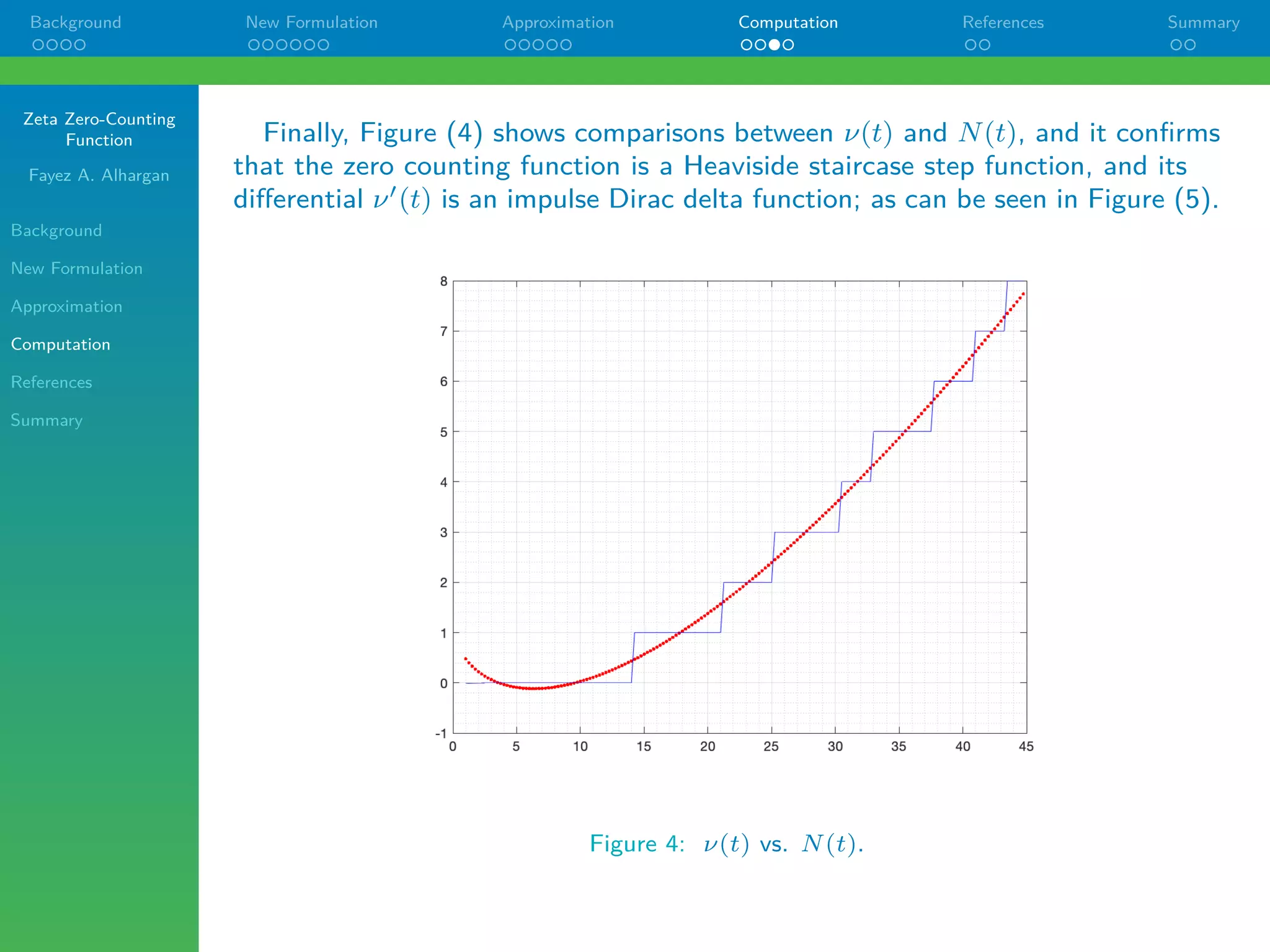
Figure (4), this vital component has been overlooked in the literature.
Figure 3: The sawtooth-like waveform component of ν(t).](https://image.slidesharecdn.com/zeros20210721-210808055857/75/Zeta-Zero-Counting-Function-18-2048.jpg)


![Zeta Zero-Counting
Function
Fayez A. Alhargan
Background
New Formulation
Approximation
Computation
References
Summary
Background New Formulation Approximation Computation References Summary
The Zero-Counting Function Proof on One Slide
The zero-counting function ν(t) of the number of zeros of ξ(s), in the range {s, s̄}
enclosed by the contour D, is defined as
4πiν(t) =
I
D
h
ξ0
(s)
ξ(s)
i
ds =
I
D
h
ζ0
(s)
ζ(s)
+
1
(s − 1)
+
1
s
+
Γ0
( s
2 )
Γ( s
2 )
−
1
2
ln π
i
ds.
(28)
where the closed contour D encompasses the critical strip [0 ≤ (s) ≤ 1]. Thus,
4πiν(t) =
I
L1
h
ζ0
(s)
ζ(s)
+
Γ0
( s
2 )
Γ( s
2 )
−
1
2
ln π
i
ds +
I
L2
h
1
(s − 1)
+
1
s
i
ds. (29)
Integrating, using line integral for L1 and residue theorem for L2, we have
2πiν(t) = ln ζ(s) − ln ζ(s̄) + ln Γ( s
2 ) − ln Γ( s̄
2 ) + ln π
− s
2 − ln π
− s̄
2 + 2πi. (30)
Utilizing Stirling approximation, we have
2πiν(t) =( 1
4 + i t
2 ) ln( 1
4 + i t
2 ) − ( 1
4 − i t
2 ) ln( 1
4 − i t
2 )
+ 1
2 ln( 1
4 − i t
2 ) − 1
2 ln( 1
4 + i t
2 )
+ ln ζ( 1
2 + it) − ln ζ( 1
2 − it) − it ln πe = 2πi
X
m
H(t − tm).
(31)
Q.E.D.
Fayez A. Alhargan](https://image.slidesharecdn.com/zeros20210721-210808055857/75/Zeta-Zero-Counting-Function-24-2048.jpg)


![Mathematics of nyquist plot [autosaved] [autosaved]](https://cdn.slidesharecdn.com/ss_thumbnails/mathematicsofnyquistplotautosavedautosaved-150219123133-conversion-gate02-thumbnail.jpg?width=640&height=640&fit=bounds)