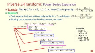
Inverse Z-Transform
Digital Signal Processing
(DSP)
Content
2
❑ Difference Equation vs Differential Equati
❑ Z-Transform
▪ Examples
▪ Properties
❑ Inverse Z-Transform
▪ Long Division
▪ Partial Fraction
Difference Equation vs Differential Equation
3
❑ A difference equation expresses the change in some variable as a result
of a finite change in the other variable.
❑ A differential equation expresses the change in some variable as a result
of an infinitesimal change in the other variable.
Z-Transform
4
❑ Difference equations can be solved using z-transforms which provide a
convenient approach for solving LTI equations.
❑ The z-transform is an important tool in the analysis and design of
discrete-time systems.
❑ It simplifies the solution of discrete-time problems by converting LTI
difference equations to algebraic equations and convolution to
multiplication.
❑ Thus, it plays a role similar to that served by Laplace transforms in
continuous-time problems.
Laplace Transform and Z-Transform
❑ Given the sampled impulse train of a signal
𝑥∗ 𝑡
𝑥∗ 𝑡 = 𝑥 0 𝛿 𝑡 + 𝑥 𝑇 𝛿 𝑡 − 𝑇 + ⋯ + 𝑥 𝑘𝑇 𝛿(𝑡 − 𝑘𝑇) + ⋯
∞
= ∑ 𝑥 𝑘𝑇 𝛿 𝑡 − 𝑘𝑇
𝑘=0 12
Laplace Transform and Z-Transform
𝑋∗ 𝑆 = 𝑥 0 + 𝑥 𝑇 𝑒−𝑠𝑇 + 𝑥 2𝑇 𝑒−𝑠2𝑇 + ⋯ + 𝑥 𝑘𝑇 𝑒−𝑠𝑘𝑇 + ⋯
∞ ∞
𝑋∗ 𝑆 = ∑ 𝑥 𝑘𝑇 𝑒−𝑠𝑘𝑇 = ∑ 𝑥 𝑘𝑇 (𝑒𝑠𝑇)−𝑘 → (1)
𝑘=0 𝑘=0
❑ The z-transform is
∞
𝑋 𝑧 = ∑ 𝑥 𝑘𝑇 𝑧−𝑘
𝑘=0
6
→ (2)
❑ Comparing (1) and (2) yields
𝑧 = 𝑒𝑠𝑇 where 𝑇 is the sample period
A Note
❑ In general, given a transfer function in s-domain you cannot just replace
𝑠 by s = 𝑙𝑛𝑧
(from 𝑧 = 𝑒𝑠𝑇) to get its z-domain transfer function.
7
𝑇
❑ The reason is that 𝑧 = 𝑒𝑠𝑇 is true with the sampled signal.
Identities Used Repeatedly
1
1 − 𝑎
, 𝑎 < 1
∞
∑ 𝑎𝑘 =
𝑘=0
𝑛
∑ 𝑎𝑘 =
𝑘=0
1 − 𝑎𝑛+1
1 − 𝑎
, 𝑎 = 1
❑ Special Cases:
∞
∑ 𝑘𝑎𝑘 =
𝑘=0
1
(1 − 𝑎)2
, 𝑎 < 1
8
Signal, 𝐱(𝒌𝑻) Z-Transform, 𝐗(𝐳) Z-Transform, 𝐗(𝐳) ROC
1 ✿(𝒌𝑻) 1 1 all Z
2 ✿(𝒌𝑻 − 𝒒) 𝐳−𝒒 𝐳−𝒒
𝐳 ≠ 𝟎
3 𝐮(𝒌𝑻)
𝟏
𝟏 − 𝒛−𝟏
𝐳
𝐳 − 𝟏
𝐳 > 𝟏
4 𝐚𝒌 𝐮(𝐤𝐓)
𝟏
𝟏 − 𝒂𝒛−𝟏
𝐳
𝐳 − 𝐚
𝐳 > 𝐚
5 𝒌 𝐮(𝐤𝐓)
𝟏
(𝟏 − 𝒛−𝟏)𝟐
𝐳
(𝐳 − 𝟏)𝟐
𝐳 > 𝟏
6 𝒌 𝐚𝒌 𝐮(𝐤𝐓)
𝐚𝒛−𝟏
(𝟏 − 𝐚𝒛−𝟏)𝟐
𝐚𝐳
(𝐳 − 𝐚)𝟐
𝐳 > 𝐚
7 𝐜𝐨𝐬(𝜔𝟎𝐤𝐓)
𝟏 − 𝒛−𝟏𝐜𝐨𝐬(𝜔𝟎)
𝟏 − 𝟐𝒛−𝟏 𝐜𝐨𝐬 𝜔𝟎 + 𝒛−𝟐
𝐳𝟐 − 𝐳𝐜𝐨𝐬(𝜔𝟎)
𝐳𝟐 − 𝟐𝐳 𝐜𝐨𝐬 𝜔𝟎 + 𝟏
𝐳 > 𝟏
8 𝐬𝐢𝐧(𝜔𝟎𝐤𝐓)
𝒛−𝟏𝐬𝐢𝐧(𝜔𝟎)
𝟏 − 𝟐𝒛−𝟏 𝐜𝐨𝐬 𝜔𝟎 + 𝒛−𝟐
𝐳 𝐬𝐢𝐧(𝜔𝟎)
𝐳𝟐 − 𝟐𝐳 𝐜𝐨𝐬 𝜔𝟎 + 𝟏
𝐳 > 𝟏
9 𝐫𝒌 𝐜𝐨𝐬(𝜔𝟎𝐤𝐓)
𝟏 − 𝐫 𝒛−𝟏𝐜𝐨𝐬(𝜔𝟎)
𝟏 − 𝟐𝐫 𝒛−𝟏 𝐜𝐨𝐬 𝜔𝟎 + 𝐫𝟐 𝒛−𝟐
𝐳𝟐 − 𝒓 𝐳 𝐜𝐨𝐬(𝜔𝟎)
𝐳𝟐 − 𝟐𝒓 𝐳 𝐜𝐨𝐬 𝜔𝟎 + 𝐫𝟐
𝐳 > 𝐫
10 𝐫𝒌 𝐬𝐢𝐧(𝜔𝟎𝐤𝐓)
𝒓 𝒛−𝟏𝐬𝐢𝐧(𝜔𝟎)
𝟏 − 𝟐𝐫 𝒛−𝟏 𝐜𝐨𝐬 𝜔𝟎 + 𝐫𝟐 𝒛−𝟐
𝒓 𝐳 𝐬𝐢𝐧(𝜔𝟎)
𝐳𝟐 − 𝟐𝒓 𝐳 𝐜𝐨𝐬 𝜔𝟎 + 𝐫𝟐
𝐳 > 𝐫
9
The inverse Z-Transform
10
The Inverse Z-Transform
❑ Formal inverse z-transform is based on a Cauchy integral
❑ Less formal ways sufficient most of the time
1) Direct or Long Division Method
2) Partial fraction expansion and Look-up Table
3) Inversion Integral Method (Residue-theorem)
x(kT)= Z −1
X (z)=
1
 X (z)zk−1
dz
2j C
11
Inverse Z-Transform: Power Series Expansion
12
❑ Using Long Division to expand X(z) as a series

X (z)= x(0)+ x(T )z−1
+ x(2T)z−2
+... = x(kT)z−k
k=0
❑ Write the inverse transform as the sequence
x(kT)={x(0), x(T), x(2T),...}
Inverse Z-Transform: Power Series Expansion
❑ Solution:
−1
35
z −1)(z − 0.2)
10z + 5
❑ Example: Find x(n) for n = 0, 1, 2, 3, 4, when X(z) is given by: X (z)=
(
−2
1−1.2z−1
+ 0.2z
10z−1
+5z−2
X (z)=
▪ First, rewrite X(z) as a ratio of polynomial in 𝑧 , as follows:
▪ Dividing the numerator by the denominator, we have:
10z−1
+17z−2
+18.4z−3
+18.68z−4
1−1.2z−1
+ 0.2z−2
10z−1
+ 5z−2
17z−2
− 2z−3
17z−2
− 20.4z−3
+ 3.4z−4
18.4z−3
−3.4z−4
18.4z−3
− 22.08z−4
+ 3.68z−5
18.68z−4
−3.68z−5
18.68z−4
− 22.416z−5
+ 3.736z−6
10z−1
−12z−2
+ 2z−3 Therefore,
• x(0) = 0,
• x(1) = 10,
• x(2) = 17,
• x(3) = 18.4
• x(4) = 18.68
Home work : 3.10 , 3.11, 3.13 (a, b c, d)

Digital Signal Processing (DSP) Inverse Z-Transform

  • 1.
  • 2.
    Content 2 ❑ Difference Equationvs Differential Equati ❑ Z-Transform ▪ Examples ▪ Properties ❑ Inverse Z-Transform ▪ Long Division ▪ Partial Fraction
  • 3.
    Difference Equation vsDifferential Equation 3 ❑ A difference equation expresses the change in some variable as a result of a finite change in the other variable. ❑ A differential equation expresses the change in some variable as a result of an infinitesimal change in the other variable.
  • 4.
    Z-Transform 4 ❑ Difference equationscan be solved using z-transforms which provide a convenient approach for solving LTI equations. ❑ The z-transform is an important tool in the analysis and design of discrete-time systems. ❑ It simplifies the solution of discrete-time problems by converting LTI difference equations to algebraic equations and convolution to multiplication. ❑ Thus, it plays a role similar to that served by Laplace transforms in continuous-time problems.
  • 5.
    Laplace Transform andZ-Transform ❑ Given the sampled impulse train of a signal 𝑥∗ 𝑡 𝑥∗ 𝑡 = 𝑥 0 𝛿 𝑡 + 𝑥 𝑇 𝛿 𝑡 − 𝑇 + ⋯ + 𝑥 𝑘𝑇 𝛿(𝑡 − 𝑘𝑇) + ⋯ ∞ = ∑ 𝑥 𝑘𝑇 𝛿 𝑡 − 𝑘𝑇 𝑘=0 12
  • 6.
    Laplace Transform andZ-Transform 𝑋∗ 𝑆 = 𝑥 0 + 𝑥 𝑇 𝑒−𝑠𝑇 + 𝑥 2𝑇 𝑒−𝑠2𝑇 + ⋯ + 𝑥 𝑘𝑇 𝑒−𝑠𝑘𝑇 + ⋯ ∞ ∞ 𝑋∗ 𝑆 = ∑ 𝑥 𝑘𝑇 𝑒−𝑠𝑘𝑇 = ∑ 𝑥 𝑘𝑇 (𝑒𝑠𝑇)−𝑘 → (1) 𝑘=0 𝑘=0 ❑ The z-transform is ∞ 𝑋 𝑧 = ∑ 𝑥 𝑘𝑇 𝑧−𝑘 𝑘=0 6 → (2) ❑ Comparing (1) and (2) yields 𝑧 = 𝑒𝑠𝑇 where 𝑇 is the sample period
  • 7.
    A Note ❑ Ingeneral, given a transfer function in s-domain you cannot just replace 𝑠 by s = 𝑙𝑛𝑧 (from 𝑧 = 𝑒𝑠𝑇) to get its z-domain transfer function. 7 𝑇 ❑ The reason is that 𝑧 = 𝑒𝑠𝑇 is true with the sampled signal.
  • 8.
    Identities Used Repeatedly 1 1− 𝑎 , 𝑎 < 1 ∞ ∑ 𝑎𝑘 = 𝑘=0 𝑛 ∑ 𝑎𝑘 = 𝑘=0 1 − 𝑎𝑛+1 1 − 𝑎 , 𝑎 = 1 ❑ Special Cases: ∞ ∑ 𝑘𝑎𝑘 = 𝑘=0 1 (1 − 𝑎)2 , 𝑎 < 1 8
  • 9.
    Signal, 𝐱(𝒌𝑻) Z-Transform,𝐗(𝐳) Z-Transform, 𝐗(𝐳) ROC 1 ✿(𝒌𝑻) 1 1 all Z 2 ✿(𝒌𝑻 − 𝒒) 𝐳−𝒒 𝐳−𝒒 𝐳 ≠ 𝟎 3 𝐮(𝒌𝑻) 𝟏 𝟏 − 𝒛−𝟏 𝐳 𝐳 − 𝟏 𝐳 > 𝟏 4 𝐚𝒌 𝐮(𝐤𝐓) 𝟏 𝟏 − 𝒂𝒛−𝟏 𝐳 𝐳 − 𝐚 𝐳 > 𝐚 5 𝒌 𝐮(𝐤𝐓) 𝟏 (𝟏 − 𝒛−𝟏)𝟐 𝐳 (𝐳 − 𝟏)𝟐 𝐳 > 𝟏 6 𝒌 𝐚𝒌 𝐮(𝐤𝐓) 𝐚𝒛−𝟏 (𝟏 − 𝐚𝒛−𝟏)𝟐 𝐚𝐳 (𝐳 − 𝐚)𝟐 𝐳 > 𝐚 7 𝐜𝐨𝐬(𝜔𝟎𝐤𝐓) 𝟏 − 𝒛−𝟏𝐜𝐨𝐬(𝜔𝟎) 𝟏 − 𝟐𝒛−𝟏 𝐜𝐨𝐬 𝜔𝟎 + 𝒛−𝟐 𝐳𝟐 − 𝐳𝐜𝐨𝐬(𝜔𝟎) 𝐳𝟐 − 𝟐𝐳 𝐜𝐨𝐬 𝜔𝟎 + 𝟏 𝐳 > 𝟏 8 𝐬𝐢𝐧(𝜔𝟎𝐤𝐓) 𝒛−𝟏𝐬𝐢𝐧(𝜔𝟎) 𝟏 − 𝟐𝒛−𝟏 𝐜𝐨𝐬 𝜔𝟎 + 𝒛−𝟐 𝐳 𝐬𝐢𝐧(𝜔𝟎) 𝐳𝟐 − 𝟐𝐳 𝐜𝐨𝐬 𝜔𝟎 + 𝟏 𝐳 > 𝟏 9 𝐫𝒌 𝐜𝐨𝐬(𝜔𝟎𝐤𝐓) 𝟏 − 𝐫 𝒛−𝟏𝐜𝐨𝐬(𝜔𝟎) 𝟏 − 𝟐𝐫 𝒛−𝟏 𝐜𝐨𝐬 𝜔𝟎 + 𝐫𝟐 𝒛−𝟐 𝐳𝟐 − 𝒓 𝐳 𝐜𝐨𝐬(𝜔𝟎) 𝐳𝟐 − 𝟐𝒓 𝐳 𝐜𝐨𝐬 𝜔𝟎 + 𝐫𝟐 𝐳 > 𝐫 10 𝐫𝒌 𝐬𝐢𝐧(𝜔𝟎𝐤𝐓) 𝒓 𝒛−𝟏𝐬𝐢𝐧(𝜔𝟎) 𝟏 − 𝟐𝐫 𝒛−𝟏 𝐜𝐨𝐬 𝜔𝟎 + 𝐫𝟐 𝒛−𝟐 𝒓 𝐳 𝐬𝐢𝐧(𝜔𝟎) 𝐳𝟐 − 𝟐𝒓 𝐳 𝐜𝐨𝐬 𝜔𝟎 + 𝐫𝟐 𝐳 > 𝐫 9
  • 10.
  • 11.
    The Inverse Z-Transform ❑Formal inverse z-transform is based on a Cauchy integral ❑ Less formal ways sufficient most of the time 1) Direct or Long Division Method 2) Partial fraction expansion and Look-up Table 3) Inversion Integral Method (Residue-theorem) x(kT)= Z −1 X (z)= 1  X (z)zk−1 dz 2j C 11
  • 12.
    Inverse Z-Transform: PowerSeries Expansion 12 ❑ Using Long Division to expand X(z) as a series  X (z)= x(0)+ x(T )z−1 + x(2T)z−2 +... = x(kT)z−k k=0 ❑ Write the inverse transform as the sequence x(kT)={x(0), x(T), x(2T),...}
  • 13.
    Inverse Z-Transform: PowerSeries Expansion ❑ Solution: −1 35 z −1)(z − 0.2) 10z + 5 ❑ Example: Find x(n) for n = 0, 1, 2, 3, 4, when X(z) is given by: X (z)= ( −2 1−1.2z−1 + 0.2z 10z−1 +5z−2 X (z)= ▪ First, rewrite X(z) as a ratio of polynomial in 𝑧 , as follows: ▪ Dividing the numerator by the denominator, we have: 10z−1 +17z−2 +18.4z−3 +18.68z−4 1−1.2z−1 + 0.2z−2 10z−1 + 5z−2 17z−2 − 2z−3 17z−2 − 20.4z−3 + 3.4z−4 18.4z−3 −3.4z−4 18.4z−3 − 22.08z−4 + 3.68z−5 18.68z−4 −3.68z−5 18.68z−4 − 22.416z−5 + 3.736z−6 10z−1 −12z−2 + 2z−3 Therefore, • x(0) = 0, • x(1) = 10, • x(2) = 17, • x(3) = 18.4 • x(4) = 18.68
  • 16.
    Home work :3.10 , 3.11, 3.13 (a, b c, d)