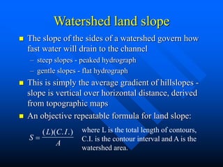
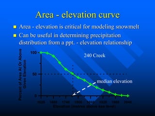
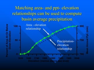
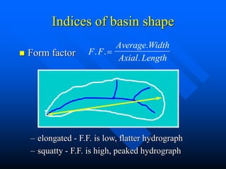
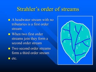
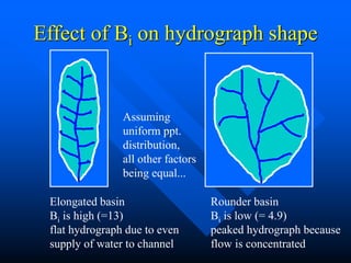
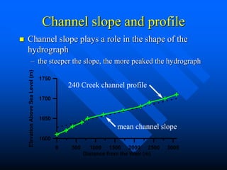
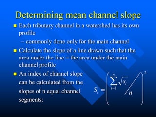
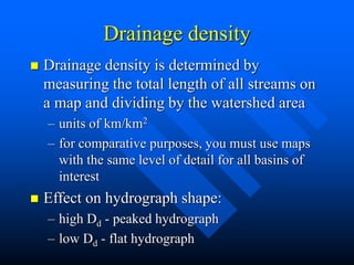
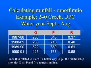
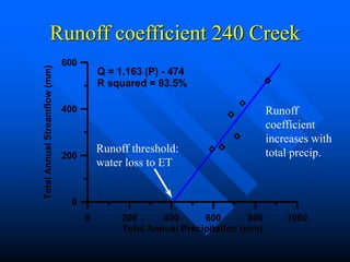
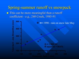
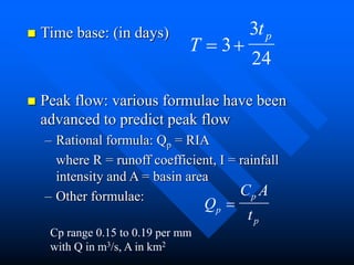
Basic Hydrology
Precipitation - Runoff Relations
Watershed Morphology
Watershed morphology
 Morphological properties of a watershed
can affect the shape of the storm
hydrograph and the delivery of sediment to
the main channel
 Various parameters can be calculated to
describe the channel network and the
physical characteristics of the watershed
– these all affect hydrograph shape
Basin size
 Delineate watershed according to the height
of land that separates water draining to the
point of interest from water that drains to
adjacent basins
 Watershed area (km2, ha)
– smaller watersheds tend to have a more peaked
hydrograph, more intermittent water supply
– larger watersheds have flatter hydrographs
because larger channel network can store more
water
Watershed land slope
 The slope of the sides of a watershed govern how
fast water will drain to the channel
– steep slopes - peaked hydrograph
– gentle slopes - flat hydrograph
 This is simply the average gradient of hillslopes -
slope is vertical over horizontal distance, derived
from topographic maps
 An objective repeatable formula for land slope:
S
L C I
A

( )( . .) where L is the total length of contours,
C.I. is the contour interval and A is the
watershed area.
Area - elevation curve
 Area - elevation is critical for modeling snowmelt
 Can be useful in determining precipitation
distribution from a ppt. - elevation relationship
1620 1680 1740 1800 1860 1920 1980 2040
Elevation (metres above sea level)
0
50
100
Percent
of
Area
At
Or
Above
Given
Elevation
240 Creek
median elevation
Matching area- and ppt- elevation
relationships can be used to compute
basin average precipitation
1620 1680 1740 1800 1860 1920 1980 2040
Elevation (metres above sea level)
0
50
100
Percent
of
Area
At
Or
Below
Given
Elevation
700
750
800
Mean
Annual
Ppt.
(mm)
Precipitation-
elevation
relationship
Area - elevation
relationship
Indices of basin shape
 Form factor
– elongated - F.F. is low, flatter hydrograph
– squatty - F.F. is high, peaked hydrograph
F F
Average Width
Axial Length
. .
.
.

Strahler’s order of streams
 A headwater stream with no
tributaries is a first order
stream
 When two first order
streams join they form a
second order stream
 Two second order streams
form a third order stream
 etc.
1
1
2
2
1
1 1
2 1
1
2
3
3
1
Bifurcation ratio
 Bi = ratio of # first order to # second order streams
 If watershed is > 2nd order:
1 2 3
Stream Order u
0.5
1.0
1.5
2.0
2.5
log
(#
Streams
of
Order
u)
log (Nu) = 2.77 -0.693 (u)
Plot log Nu vs. u as shown, Bi is the anti-log
of the slope of the regression line. For the
example given, Bi = anti-log(0.693) = 4.93
Effect of Bi on hydrograph shape
Elongated basin
Bi is high (=13)
flat hydrograph due to even
supply of water to channel
Rounder basin
Bi is low (= 4.9)
peaked hydrograph because
flow is concentrated
Assuming
uniform ppt.
distribution,
all other factors
being equal...
Channel slope and profile
 Channel slope plays a role in the shape of the
hydrograph
– the steeper the slope, the more peaked the hydrograph
0 500 1000 1500 2000 2500 3000
Distance from the Weir (m)
1600
1650
1700
1750
Elevation
Above
Sea
Level
(m)
240 Creek channel profile
mean channel slope
Determining mean channel slope
 Each tributary channel in a watershed has its own
profile
– commonly done only for the main channel
 Calculate the slope of a line drawn such that the
area under the line = the area under the main
channel profile
 An index of channel slope
can be calculated from the
slopes of n equal channel
segments:
S
s
n
c
i
i
n















1
2
Drainage density
 Drainage density is determined by
measuring the total length of all streams on
a map and dividing by the watershed area
– units of km/km2
– for comparative purposes, you must use maps
with the same level of detail for all basins of
interest
 Effect on hydrograph shape:
– high Dd - peaked hydrograph
– low Dd - flat hydrograph
Valley flat
 Area adjacent to stream or river floodplain
where the slope is < 8%
 Buffers the stream channel from landslides
which may run out on the valley flat before
depositing sediment in the channel.
 Calculate the length of mainstem channel
that has a valley flat, express as a proportion
of the length of the mainstem channel.
Other factors
 Lithology
– importance: can govern slope stability, bedrock
leakage, permeability
 Presence or absence of glaciers
– will govern timing and mangitude of peak
runoff
 Land use...
Precipitation - runoff
 Methods have been developed to predict
characteristics of runoff as a function of
precipitation characteristics
– volume of runoff
» seasonal
» annual
» based on seasonal or annual total precipitation
– peak flow
» annual peak flow - e.g., snowmelt peak (interior), a
function of peak snow accumulation
» storm peaks - a function of rainfall intensity
Runoff coefficient
 Simplest form of ppt - runoff relation
– ratio of total streamflow
over total precipitation
 Runoff coefficient can be assessed annually,
seasonally or monthly depending on
purpose
 Should be a characteristic quantity of a
watershed assuming no change in land use
R
Q
P

Calculating rainfall - runoff ratio
Example: 240 Creek, UPC
Water year Sept - Aug
Q P R
1987-88 236 640 0.37
1988-89 283 713 0.40
1989-90 522 859 0.61
1990-91 425 738 0.58
Since R is related to P or Q, a better way to get the ralationship
is to plot Q vs. P and fit a regression line.
Runoff coefficient 240 Creek
0 200 400 600 800 1000
Total Annual Precipitation (mm)
0
200
400
600
Total
Annual
Streamflow
(mm)
Q = 1.163 (P) - 474
R squared = 83.5%
Runoff threshold:
water loss to ET
Runoff
coefficient
increases with
total precip.
Spring-summer runoff vs snowpack
 This can be more meaningful than a runoff
coefficient - e.g., 240 Creek, 1985-91
120 160 200 240 280 320
Snowpack, April 1 (mm)
100
200
300
400
500
Total
April
-
July
Streamflow
(mm)
Q = 1.355 (S)
R squared = 99.6%
1990 - rain on snow late May
Predicting spring runoff in
interior watersheds
 Unlike runoff coefficient relationship, relationship
between spring - summer runoff and peak
snowpack passes through the origin
– this shows that virtually all the snowpack contributes to
spring - summer runoff
 Slope > 1: relationship is a very good predictor of
snowmelt runoff but doesn’t account for
precipitation that occurs after April 1 - doesn’t
work for unusual conditions such as rain-on-snow
Precipitation & temperature
Jan Feb Mar Apr May Jun Jul Aug Sep Oct Nov Dec
0
40
80
120
Total
Monthly
Precipitation
(mm)
-20
-10
0
10
20
Mean
Monthly
Temperature
(deg
C)
Total Monthly Precipitation
Mean Monthly Max Temperature
Mean Monthly Min Temperature
Use of snow course data to
predict runoff
 For an interior watershed, snow course data should
provide a better measure of runoff
 Used to predict inflows to reservoirs, potential
floods
 For a coastal watershed, rainfall data is needed, but
annual runoff coefficient is probably relatively
meaningless
– monthly runoff ratio, averaged over several
years may be useful
– expected to be much higher than for interior w/s
Effect of antecedent conditions
on rainfall - runoff relation
 The amount of soil moisture prior to a storm will
affect the runoff ratio for that storm, and will affect
the shape of the hydrograph
– wet antecedent conditions lead to more runoff
per unit ppt., dry antecedent conditions result in
more of the input water going to basin recharge
– antecedent conditions are a function of ET and
soil/groundwater drainage.
 Not always possible to quantify these factors...
Antecedent Precipitation Index
 API is a method of accounting for daily
changes in water balance.
– API is a decay factor - each days API is a fixed
percentage of the previous day’s API (e.g.,
90%), plus daily rainfall and/or snowmelt
– runoff coefficient will vary according to the
API:
» the higher the API, the higher the runoff coefficient
API for Russell Creek Jan 1992
0 10 20 30
0
40
80
Daily
Rainfall
(mm)
0
100
200
API
(mm)
API for Russell Creek Jul 1992
0 10 20 30
0
4
8
Daily
Rainfall
(mm)
0
20
40
API
(mm)
Synthetic unit hydrograph
 It has been determined empirically that the
parameters of the unit hydrograph - lag
time, peak and time base - can be
determined from basin morphology
 lag time: (hours)
 
t C LL
p t C

0 3
.
LC
L = length of main
channel
Ct range 1.8 to 2.2
 Time base: (in days)
 Peak flow: various formulae have been
advanced to predict peak flow
– Rational formula: Qp = RIA
where R = runoff coefficient, I = rainfall
intensity and A = basin area
– Other formulae:
T
tp
 
3
3
24
Q
C A
t
p
p
p

Cp range 0.15 to 0.19 per mm
with Q in m3/s, A in km2
Russell Creek 1991 - 92
0 20 40 60 80 100
Max 24-hour Storm Intensity (mm)
0
10
20
30
40
Peak
Flow
(m3/s)
R2 = 83.8%
Peak = 0.342 (24hr) + 1.17 Base
R2 = 92 %

ws morphology7.PPT

  • 1.
    Basic Hydrology Precipitation -Runoff Relations Watershed Morphology
  • 2.
    Watershed morphology  Morphologicalproperties of a watershed can affect the shape of the storm hydrograph and the delivery of sediment to the main channel  Various parameters can be calculated to describe the channel network and the physical characteristics of the watershed – these all affect hydrograph shape
  • 3.
    Basin size  Delineatewatershed according to the height of land that separates water draining to the point of interest from water that drains to adjacent basins  Watershed area (km2, ha) – smaller watersheds tend to have a more peaked hydrograph, more intermittent water supply – larger watersheds have flatter hydrographs because larger channel network can store more water
  • 4.
    Watershed land slope The slope of the sides of a watershed govern how fast water will drain to the channel – steep slopes - peaked hydrograph – gentle slopes - flat hydrograph  This is simply the average gradient of hillslopes - slope is vertical over horizontal distance, derived from topographic maps  An objective repeatable formula for land slope: S L C I A  ( )( . .) where L is the total length of contours, C.I. is the contour interval and A is the watershed area.
  • 5.
    Area - elevationcurve  Area - elevation is critical for modeling snowmelt  Can be useful in determining precipitation distribution from a ppt. - elevation relationship 1620 1680 1740 1800 1860 1920 1980 2040 Elevation (metres above sea level) 0 50 100 Percent of Area At Or Above Given Elevation 240 Creek median elevation
  • 6.
    Matching area- andppt- elevation relationships can be used to compute basin average precipitation 1620 1680 1740 1800 1860 1920 1980 2040 Elevation (metres above sea level) 0 50 100 Percent of Area At Or Below Given Elevation 700 750 800 Mean Annual Ppt. (mm) Precipitation- elevation relationship Area - elevation relationship
  • 7.
    Indices of basinshape  Form factor – elongated - F.F. is low, flatter hydrograph – squatty - F.F. is high, peaked hydrograph F F Average Width Axial Length . . . . 
  • 8.
    Strahler’s order ofstreams  A headwater stream with no tributaries is a first order stream  When two first order streams join they form a second order stream  Two second order streams form a third order stream  etc. 1 1 2 2 1 1 1 2 1 1 2 3 3 1
  • 9.
    Bifurcation ratio  Bi= ratio of # first order to # second order streams  If watershed is > 2nd order: 1 2 3 Stream Order u 0.5 1.0 1.5 2.0 2.5 log (# Streams of Order u) log (Nu) = 2.77 -0.693 (u) Plot log Nu vs. u as shown, Bi is the anti-log of the slope of the regression line. For the example given, Bi = anti-log(0.693) = 4.93
  • 10.
    Effect of Bion hydrograph shape Elongated basin Bi is high (=13) flat hydrograph due to even supply of water to channel Rounder basin Bi is low (= 4.9) peaked hydrograph because flow is concentrated Assuming uniform ppt. distribution, all other factors being equal...
  • 11.
    Channel slope andprofile  Channel slope plays a role in the shape of the hydrograph – the steeper the slope, the more peaked the hydrograph 0 500 1000 1500 2000 2500 3000 Distance from the Weir (m) 1600 1650 1700 1750 Elevation Above Sea Level (m) 240 Creek channel profile mean channel slope
  • 12.
    Determining mean channelslope  Each tributary channel in a watershed has its own profile – commonly done only for the main channel  Calculate the slope of a line drawn such that the area under the line = the area under the main channel profile  An index of channel slope can be calculated from the slopes of n equal channel segments: S s n c i i n                1 2
  • 13.
    Drainage density  Drainagedensity is determined by measuring the total length of all streams on a map and dividing by the watershed area – units of km/km2 – for comparative purposes, you must use maps with the same level of detail for all basins of interest  Effect on hydrograph shape: – high Dd - peaked hydrograph – low Dd - flat hydrograph
  • 14.
    Valley flat  Areaadjacent to stream or river floodplain where the slope is < 8%  Buffers the stream channel from landslides which may run out on the valley flat before depositing sediment in the channel.  Calculate the length of mainstem channel that has a valley flat, express as a proportion of the length of the mainstem channel.
  • 15.
    Other factors  Lithology –importance: can govern slope stability, bedrock leakage, permeability  Presence or absence of glaciers – will govern timing and mangitude of peak runoff  Land use...
  • 16.
    Precipitation - runoff Methods have been developed to predict characteristics of runoff as a function of precipitation characteristics – volume of runoff » seasonal » annual » based on seasonal or annual total precipitation – peak flow » annual peak flow - e.g., snowmelt peak (interior), a function of peak snow accumulation » storm peaks - a function of rainfall intensity
  • 17.
    Runoff coefficient  Simplestform of ppt - runoff relation – ratio of total streamflow over total precipitation  Runoff coefficient can be assessed annually, seasonally or monthly depending on purpose  Should be a characteristic quantity of a watershed assuming no change in land use R Q P 
  • 18.
    Calculating rainfall -runoff ratio Example: 240 Creek, UPC Water year Sept - Aug Q P R 1987-88 236 640 0.37 1988-89 283 713 0.40 1989-90 522 859 0.61 1990-91 425 738 0.58 Since R is related to P or Q, a better way to get the ralationship is to plot Q vs. P and fit a regression line.
  • 19.
    Runoff coefficient 240Creek 0 200 400 600 800 1000 Total Annual Precipitation (mm) 0 200 400 600 Total Annual Streamflow (mm) Q = 1.163 (P) - 474 R squared = 83.5% Runoff threshold: water loss to ET Runoff coefficient increases with total precip.
  • 20.
    Spring-summer runoff vssnowpack  This can be more meaningful than a runoff coefficient - e.g., 240 Creek, 1985-91 120 160 200 240 280 320 Snowpack, April 1 (mm) 100 200 300 400 500 Total April - July Streamflow (mm) Q = 1.355 (S) R squared = 99.6% 1990 - rain on snow late May
  • 21.
    Predicting spring runoffin interior watersheds  Unlike runoff coefficient relationship, relationship between spring - summer runoff and peak snowpack passes through the origin – this shows that virtually all the snowpack contributes to spring - summer runoff  Slope > 1: relationship is a very good predictor of snowmelt runoff but doesn’t account for precipitation that occurs after April 1 - doesn’t work for unusual conditions such as rain-on-snow
  • 22.
    Precipitation & temperature JanFeb Mar Apr May Jun Jul Aug Sep Oct Nov Dec 0 40 80 120 Total Monthly Precipitation (mm) -20 -10 0 10 20 Mean Monthly Temperature (deg C) Total Monthly Precipitation Mean Monthly Max Temperature Mean Monthly Min Temperature
  • 23.
    Use of snowcourse data to predict runoff  For an interior watershed, snow course data should provide a better measure of runoff  Used to predict inflows to reservoirs, potential floods  For a coastal watershed, rainfall data is needed, but annual runoff coefficient is probably relatively meaningless – monthly runoff ratio, averaged over several years may be useful – expected to be much higher than for interior w/s
  • 24.
    Effect of antecedentconditions on rainfall - runoff relation  The amount of soil moisture prior to a storm will affect the runoff ratio for that storm, and will affect the shape of the hydrograph – wet antecedent conditions lead to more runoff per unit ppt., dry antecedent conditions result in more of the input water going to basin recharge – antecedent conditions are a function of ET and soil/groundwater drainage.  Not always possible to quantify these factors...
  • 25.
    Antecedent Precipitation Index API is a method of accounting for daily changes in water balance. – API is a decay factor - each days API is a fixed percentage of the previous day’s API (e.g., 90%), plus daily rainfall and/or snowmelt – runoff coefficient will vary according to the API: » the higher the API, the higher the runoff coefficient
  • 26.
    API for RussellCreek Jan 1992 0 10 20 30 0 40 80 Daily Rainfall (mm) 0 100 200 API (mm)
  • 27.
    API for RussellCreek Jul 1992 0 10 20 30 0 4 8 Daily Rainfall (mm) 0 20 40 API (mm)
  • 28.
    Synthetic unit hydrograph It has been determined empirically that the parameters of the unit hydrograph - lag time, peak and time base - can be determined from basin morphology  lag time: (hours)   t C LL p t C  0 3 . LC L = length of main channel Ct range 1.8 to 2.2
  • 29.
     Time base:(in days)  Peak flow: various formulae have been advanced to predict peak flow – Rational formula: Qp = RIA where R = runoff coefficient, I = rainfall intensity and A = basin area – Other formulae: T tp   3 3 24 Q C A t p p p  Cp range 0.15 to 0.19 per mm with Q in m3/s, A in km2
  • 30.
    Russell Creek 1991- 92 0 20 40 60 80 100 Max 24-hour Storm Intensity (mm) 0 10 20 30 40 Peak Flow (m3/s) R2 = 83.8% Peak = 0.342 (24hr) + 1.17 Base R2 = 92 %