This document provides instructions for using ANSYS to analyze a plate structure with pinned connections. It describes 20 steps to: 1) import the CAD model, define materials and mesh the midplane surfaces; 2) apply multi-point constraints (MPCs) at pinned connections and a beam element between plates; 3) apply boundary conditions and a pressure load; and 4) solve and inspect results including stresses and reactions at supports. The goal is to demonstrate using MPCs to model pinned joints in a finite element analysis.

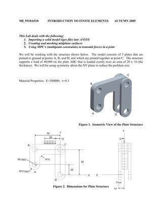
1. ME 5510/6510 INTRODUCTION TO FINITE ELEMENTS AUTUMN 2005
This Lab deals with the following:
1. Importing a solid model (iges file) into ANSYS
2. Creating and meshing midplane surfaces
3. Using MPC’s (multipoint constraints) to transmit forces in a joint
We will be working with the structure shown below. The model consists of 3 plates that are
pinned to ground at points A, B, and D, and which are pinned together at point C. The structure
supports a load of 40,000 on the plate ABC that is loaded evenly over an area of 20 x 10 (the
thickness). We will be using symmetry about the XY plane to reduce the problem size.
Material Properties: E=200000; ν=0.3
B
Figure 1. Isometric View of the Plate Structure
Z
B C
Figure 2. Dimensions for Plate Structure
Y
12
5
5
A
C
D
X
Y
50
20
50
R10
R5 (typ)
R10 (typ)
A
D
10
20

2. Step 1: Import the model into Ansys
Download the iges file of the part shown above from the course website and save in your CADE
directory (home directory or other). Start ANSYS and then do the following:
FileÆImportÆIGESÆ(window)leave the default settings and select OKÆ(window) browse to
find the iges part where you saved it (the part is called “lab_part.igs”) and open it into ANSYS.
Note you can use the mouse buttons to dynamically orient the model if you pick the upper right
view menu button (hold cursor over button and it should say “Dynamic Model Mode”). Also,
use Plot and PlotCntrls to display the keypoints, lines, and volumes that are automatically
brought in with the iges model.
Step 2: Modify the model to make use of symmetry
WorkplaneÆhighlight the button “Display Working Plane”
WorkplaneÆWP Setting…Æ(window) click Grid and Triad. You may want to adjust the size,
minimum, and maximum values to 5, 20, and 20, respectively, to help display the working
planeÆclick OK.
PreprocessorÆModelingÆOperate ÆBooleansÆDivideÆVolume by wrkplaneÆ(window)
pick the center plate volumeÆOKÆPartitions the volume down the center into 2 volumes.
PreprocessorÆModelingÆDelete ÆVolume and belowÆ (window) pick the volumes forward
of the XY plane (i.e. the front plate and the front half of the center plate), then hit OKÆvolumes
are deleted.
Step 3: Partition the rear vertical plate to create a midsurface (area)
WorkplaneÆoffset WP by incrementsÆ(window) type 0,0,-9.5 in the X,Y,Z offsets box and hit
OK.
PreprocessorÆModelingÆOperate ÆBooleansÆDivideÆVolume by wrkplaneÆ(window)
pick the rear vertical plate volume, then hit OKÆPartitions the volume down the center into 2
volumes.
Step 4: Select and Display only the areas (midplanes) we will be concerned with
SelectÆEntitiesÆ(window) choose Areas and By Num/Pick and then hit OKÆ(window) pick
the exposed misdsurface of the center plate and the midsurface of the rear vertical plate which
you just created.
Plot the areas (or simply type “aplot” in the command prompt); you should see the only the 2
midplanes we are concerned with.
Step 5: More Work Plane manipulation and partitioning of the areas for meshing and
loading purposes. You may want to look at the figure below as a guide for what the final
partitions should look like.
WorkplaneÆAlign WP withÆGlobal Cartesian (you may need to replote to see effect).

3. WorkplaneÆoffset WP by incrementsÆ(window) adjust the degrees sensitivity to 90 by sliding
button, then hit the +Y button once, and then hit the X- button once.
PreprocessorÆModelingÆOperate ÆBooleansÆDivideÆArea by wrkplaneÆ(window) pick
the rear vertical plate area, then hit OK.
WorkplaneÆoffset WP by incrementsÆ(window) type 0,0,10 in the X,Y,Z offsets box and hit
OK.
PreprocessorÆModelingÆOperate ÆBooleansÆDivideÆArea by wrkplaneÆ(window) pick
the rear vertical plate area, then hit OK.
WorkplaneÆoffset WP by incrementsÆ(window) type 0,0,30 in the X,Y,Z offsets box and hit
OK.
PreprocessorÆModelingÆOperate ÆBooleansÆDivideÆArea by wrkplaneÆ(window) pick
the rear vertical plate area, then hit OK.
ETC….
Keep partitioning the areas until you have what you see below. Remember that you can always
realign the work plane to the global coordinate system in case you loose track of the Work Plane
orientation.
Figure 3. Partitioned Midplane Areas

4. Step 6: Define Material Properties
PreprocessorÆMaterial PropertiesÆMaterial ModelsÆ(window) double click
Structural/Linear/Elastic/IsotropicÆ(window) input modulus and Poisson’s ratioÆOKÆ(close
Material Model window).
Step 7: Define Element Type 1 (for shell elements)
PreprocessorÆElement TypeÆAdd/Edit/DeleteÆ(window) Add…Æ(window) highlight
Shell63ÆOKÆCLOSE.
Step 8: Define Physical Property Set 1 (thickness for shell63 elements)
PreprocessorÆRealConstantsÆAdd/Edit/Delete Æ(window) Add…Æ(window with element
Shell63 highlighted) OKÆ(window) input thickness of 5 (because we have constant thickness,
only the first value is required)ÆOKÆCLOSE.
(Note that because we are using symmetry, the middle plate will be the same thickness as the rear plate).
Step 9: Select and Display only the lines we will be concerned with
SelectÆEntitiesÆ(window) choose Lines and Attached to, then select Areas and hit
OKÆ(window) pick the areas on screen or just select Pick All (since we previously filtered our
areas to just these midsurfaces) and then hit OK.
Step 10: Use the Mesh Tool to set up element divisions on lines and mesh the areas
PreprocessorÆMeshingÆMesh Tool Æ(window) under element attributes, set the button to
Area, then hit SetÆ(window) select the Pick AllÆ(window) shows material properties, real
constant sets, and element type that we are going to be applying to the areas; hit OK. Now the
Mesh Tool should still be up (if not just select it again from commands). Use the Set button
under the Size Controls, Lines option to assign the element divisions shown in Figure 4 below:
5
5
25
5
5
5
5
5
5
5
5
5
5
5
25 25
5
5
5
5
5
5
5
5
5
10
10
10
5
5
5
5
10
5
5
10
10
10
10
5
5
5
5
5
5
5
5
5
5
5
5
Figure 4. Divisions Applied to Lines for Mesh Control

5. After you have assigned all the element divisions to the lines, go back to the Mesh Tool and
select that you want to mesh Areas, using a Quad shape and Free, then select MeshÆ(window)
hit the Pick All button to mesh all the areas. The resulting mesh should look something like this:
Figure 5. Mesh of the Plate Midsurfaces
Step 11: Define the MPC (Multi-Point Constraint) Element (Type 2)
PreprocessorÆElement TypeÆAdd/Edit/DeleteÆ(window) Add…Æ(window) highlight
Constraint, MPC184ÆOKÆselect the Options buttonÆ(window) set the element behavior to be
a Rigid Beam, then hit OKÆCLOSE.
(Note that there are not real constants or materials associated with an MPC)
Step 12: Define the Beam 44 Element (Type 3)
PreprocessorÆElement TypeÆAdd/Edit/DeleteÆ(window) Add…Æ(window) highlight Beam,
tapered 44 (Beam44)ÆOKÆ(Back to window, make sure Beam44 is highlighted) select
OptionsÆ(window) change “member force + moment output” to Include Output; select buttons
Rotx for stiffness release at either node I or J, but not both; then select OKÆCLOSE.

6. Step 13: Define Physical Property Set 2 (for the Beam 44)
PreprocessorÆRealConstantsÆAdd/Edit/Delete Æ(window) Add…Æ(window with element
Type Beam4 highlighted) OKÆ(window) input properties for beam element*ÆOKÆCLOSE.
* Use the following inputs for the beam element:
A= 76.5 (at both ends)
I=490.87 (at both ends in both directions)
J=981.75 (at both ends in both directions)
Step 14: Define Nodes at Centers of the Pin Holes
Create the following nodes with the given coordinates:
Node x y z
10000 0 0 -9.5
10001 0 50 -9.5
10002 0 50 0
10003 -50 20 0
10004 -50 50 0
Step 15: Build MPC’s Between the Hole Center Nodes to Hole Perimeter Nodes
PreprocessorÆModelingÆCreateÆElementsÆElement AttributesÆ(window) change Element
No. to 2, then select OK.
(you may want to zoom in on a pin hole and display only the nodes before doing the next step)
PreprocessorÆModelingÆCreateÆElementsÆAuto NumberedÆThru NodesÆ(window) select
the center node first and then a node from the ring of perimeter nodes around it, then hit Apply.
Repeat until you have created a “pinwheel” of MPC elements from the center node out to the
hole perimeter nodes. Then repeat this process for the other holes in the model. After you are
finished, your model should look as follows:
Figure 6. Mesh Including MPC’s at the Holes

7. Step 16: Build the Beam 44 Element Between the Plates
PreprocessorÆModelingÆCreateÆElementsÆElement AttributesÆ(window) change Element
No. to 3, then select OK.
PreprocessorÆModelingÆCreateÆElementsÆAuto NumberedÆThru NodesÆ(window) select
the center nodes from both plates at joint C, then select OK.
Step 17: Apply Bounday Conditions
PreprocessorÆLoadsÆDefine LoadsÆApplyÆStructuralÆDisplacementÆOn
NodesÆ(window) pick nodes 10002 and 10003, then select OKÆ(window) highlight Ux and
Uy; make sure it shows Apply As: Constant Value; enter value as 0, select OK.
PreprocessorÆLoadsÆDefine LoadsÆApplyÆStructuralÆDisplacementÆOn
NodesÆ(window) pick node 10000, then select OKÆ(window) highlight Ux, Uy and Uz; make
sure it shows Apply As: Constant Value; enter value as 0, select OK.
Type the following in the command prompt to apply symmetry boundary conditions to the nodes
on the XY plane:
nsel,s,loc,z,0,0
dsym,symm,z
nsel,all
WARNING: We have constrained the model correctly, but if we tried to run it with the BC’s
we’ve applied, ANSYS would produce a fatal error resulting from Zero Pivots in the stiffness
matrix (often associated with models that are not constrained properly and have rigid body
modes). The reason for this is that we have currently overconstrained the MPC elements. One
way to think of this is that the hole center nodes are like “master” nodes that control the “slave”
nodes around the hole perimeter. Whatever dof’s we constrain at the master node, we
automatically constrain at the slave nodes. However, because we selected all the nodes along the
XY plane to apply the symmetry BC’s, we have applied constraints to both the master and slave
nodes and have therefore overconstrained the MPC’s. This causes problems for the MPC
element and will produce errors unless we do the following:
PreprocessorÆLoadsÆDefine LoadsÆDeleteÆStructuralÆDisplacementÆOn
NodesÆ(window) pick all the hole perimeter nodes for the three holes on the center plate, then
select OKÆ(window) highlight All DOF, then hit OK.
Step 18: Apply Loading to the Model
PreprocessorÆLoadsÆDefine LoadsÆApplyÆStructuralÆPressureÆOn LinesÆ(window)
pick the line representing the width of pressure area (which we created by partitioning
previously), then select OKÆ(window) enter 200, then select OK.

8. Step 19: Solve
SolutionÆSolveÆCurrent LSÆ(asks you to review summary info) select OKÆANSYS will
begin solving the problem and will post a message “Solution is done!” when it has finished.
Close message windows and go to next step.
Step 20: Inspect Results
1. Check to make sure the torque in the beam44 element is zero (i.e. select only the beam44
element and use etable,torque,smisc,4 to get the torque in the element).
2. Determine the reactions at nodes 10000, 10003, and 10004 (i.e. where the structure is
grounded) by doing the following:
First, select only nodes 10000, 10003, and 10004 (either by using SelectÆEntities in the
GUI or using the nsel command directly). Then list the reactions; the GUI path is as
follows:
General PostprocÆList ResultsÆ Reaction SolutionÆ(window) highlight All Items and
then select OK. You should get the following
NODE FX FY FZ MX MY MZ
10000 -0.11344E-04 1653.0 38.545
10003 1245.1 868.85 -0.15373E-11 -0.67314E-11 0.53342E-11
10004 -1245.1 1478.2 0.12860E-12 -0.13020E-11 0.29280E-11
3. A contour plot of the von Mises stress should produce the following plot:
Figure 7. Contour Plot of von Mises Stress in the Plates