Downloaded 12 times
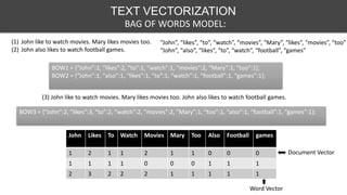
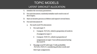
![Tokenizing:
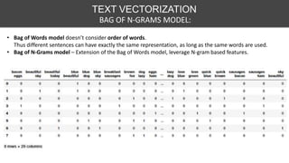
• Tokenize
• N-Grams
• Skip-Grams
• Char-grams
• Affixes (Not in example)
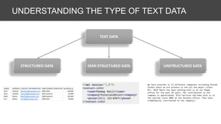
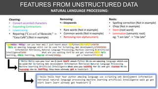
NATURAL LANGUAGE PROCESSING:
FEATURES FROM UNSTRUCTURED DATA
Enrich:
• Entity Insertion/Extraction
"Microsoft Releases Windows" -> "Microsoft(company) releases Windows(application)"
• Parse Trees
"Alice hits Bill" -> Alice/Noun_subject hits/Verb Bill/Noun_object
[('Mark', 'NNP', u'B-PERSON'), ('and', 'CC', u'O'), ('John', 'NNP', u'B-PERSON'), ('are', 'VBP', u'O'), ('working', 'VBG', u'O'),
('at', 'IN', u'O'), ('Google', 'NNP', u'B-ORGANIZATION'), ('.', '.', u'O’)]
• Reading Level](https://image.slidesharecdn.com/textfeatures-180506005643/85/Text-features-5-320.jpg)
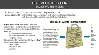
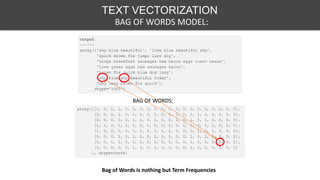
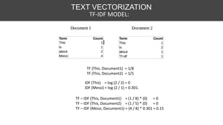
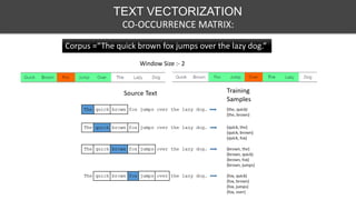
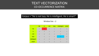
![TEXT VECTORIZATION
CO-OCCURRENCE MATRIX:
PMI = Pointwise Mutual Information.
Larger PMI Higher correlation
Where, w= word, c= context word
ISSUES: Many entries with PMI (w,c) = log 0
SOLUTION:
• Set PMI(w,c) = 0 for all unobserved pairs.
• Drop all entries of PMI< 0 [POSITIVE POINTWISE MUTUAL INFORMATION]
Produces 2 different vectors for each word:
• Describes word when it is the ‘target word’ in the window
• Describes word when it is the ‘context word’ in window](https://image.slidesharecdn.com/textfeatures-180506005643/85/Text-features-20-320.jpg)
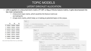
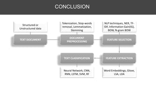


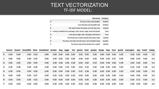
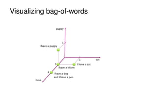
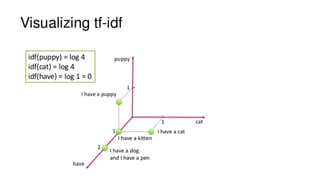
This document discusses various techniques for feature engineering on text data, including both structured and unstructured data. It covers preprocessing techniques like tokenization, stopword removal, and stemming. It then discusses methods for feature extraction, such as bag-of-words, n-grams, TF-IDF, word embeddings, topic models like LDA. It also discusses document similarity metrics and applications of feature engineered text data to text classification. The goal is to transform unstructured text into structured feature vectors that can be used for machine learning applications.