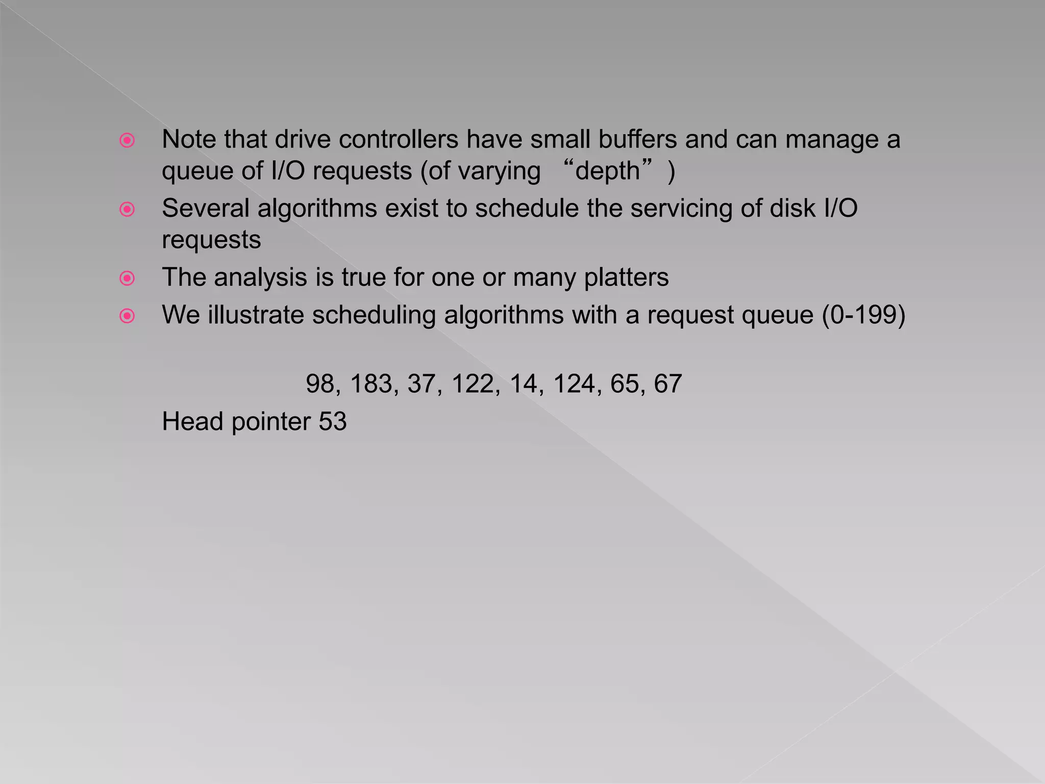
This document discusses various aspects of mass storage systems, including disk structure, disk scheduling algorithms, and operating system services for storage. It provides details on disk formatting, partitioning, and file systems. It also covers topics like swap space management, the use of raw disks versus file systems, and boot block initialization. Disk scheduling algorithms like SSTF, SCAN, C-SCAN, and LOOK are evaluated based on minimizing head movement and providing uniform wait times.

2.  Overview of Mass Storage Structure
 Disk Structure
 Disk Attachment
 Disk Scheduling
 Disk Management
 Swap-Space Management
 RAID Structure
 Stable-StorageImplementation

3. n To describe the physical structure of
secondary storage devices and its effects on
the uses of the devices
n To explain the performance characteristics of
mass-storage devices
n To evaluate disk scheduling algorithms
n To discuss operating-system services
provided for mass storage, including RAID

4.  Magnetic disks provide bulk of secondary storage of modern computers
› Drives rotate at 60 to 250 times per second
› Transfer rate is rate at which data flow between drive and computer
› Positioning time (random-access time) is time to move disk arm to
desired cylinder (seek time) and time for desired sector to rotate under
the disk head (rotational latency)
› Head crash results from disk head making contact with the disk
surface -- That’s bad
 Disks can be removable
 Drive attached to computer via I/O bus
› Busses vary, including EIDE, ATA, SATA, USB, Fibre Channel, SCSI,
SAS, Firewire
› Host controller in computer uses bus to talk to disk controller built
into drive or storage array

6.  Platters range from .85” to 14” (historically)
› Commonly 3.5”, 2.5”, and 1.8”
 Range from 30GB to 3TB per drive
 Performance
› Transfer Rate – theoretical – 6 Gb/sec
› Effective Transfer Rate – real – 1Gb/sec
› Seek time from 3ms to 12ms – 9ms common for desktop drives
› Average seek time measured or calculated based on 1/3 of tracks
› Latency based on spindle speed
 1 / (RPM / 60) = 60 / RPM
› Average latency = ½ latency

8.  Access Latency = Average access time = average seek time + average
latency
› For fastest disk 3ms + 2ms = 5ms
› For slow disk 9ms + 5.56ms = 14.56ms
 Average I/O time = average access time + (amount to transfer / transfer
rate) + controller overhead
 For example to transfer a 4KB block on a 7200 RPM disk with a 5ms
average seek time, 1Gb/sec transfer rate with a .1ms controller overhead =
› 5ms + 4.17ms + 0.1ms + transfer time =
› Transfer time = 4KB / 1Gb/s * 8Gb / GB * 1GB / 10242KB = 32 / (10242)
= 0.031 ms
› Average I/O time for 4KB block = 9.27ms + .031ms = 9.301ms

9. 1956
IBM RAMDAC computer
included the IBM Model 350
disk storage system
5M (7 bit) characters
50 x 24” platters
Access time = < 1 second

10.  Nonvolatile memory used like a hard drive
› Many technology variations
 Can be more reliable than HDDs
 More expensive per MB
 Maybe have shorter life span
 Less capacity
 But much faster
 Busses can be too slow -> connect directly to PCI for example
 No moving parts, so no seek time or rotational latency

11.  Was early secondary-storage medium
› Evolved from open spools to cartridges
 Relatively permanent and holds large quantities of data
 Access time slow
 Random access ~1000 times slower than disk
 Mainly used for backup, storage of infrequently-used data,
transfer medium between systems
 Kept in spool and wound or rewound past read-write head
 Once data under head, transfer rates comparable to disk
› 140MB/sec and greater
 200GB to 1.5TB typical storage
 Common technologies are LTO-{3,4,5} and T10000

12.  Common in large storage environments
 Multiple hosts attached to multiple storage arrays - flexible

13.  SAN is one or more storage arrays
› Connected to one or more Fibre Channel switches
 Hosts also attach to the switches
 Storage made available via LUN Masking from specific arrays
to specific servers
 Easy to add or remove storage, add new host and allocate it
storage
› Over low-latency Fibre Channel fabric
 Why have separate storage networks and communications
networks?
› Consider iSCSI, FCOE

14.  Network-attached storage (NAS) is storage made available
over a network rather than over a local connection (such as a
bus)
› Remotely attaching to file systems
 NFS and CIFS are common protocols
 Implemented via remote procedure calls (RPCs) between host
and storage over typically TCP or UDP on IP network
 iSCSI protocol uses IP network to carry the SCSI protocol
› Remotely attaching to devices (blocks)

15.  The operating system is responsible for using hardware
efficiently — for the disk drives, this means having a fast
access time and disk bandwidth
 Minimize seek time
 Seek time  seek distance
 Disk bandwidth is the total number of bytes transferred,
divided by the total time between the first request for service
and the completion of the last transfer

16.  There are many sources of disk I/O request
› OS
› System processes
› Users processes
 I/O request includes input or output mode, disk address, memory
address, number of sectors to transfer
 OS maintains queue of requests, per disk or device
 Idle disk can immediately work on I/O request, busy disk means
work must queue
› Optimization algorithms only make sense when a queue exists

17.  Note that drive controllers have small buffers and can manage a
queue of I/O requests (of varying “depth”)
 Several algorithms exist to schedule the servicing of disk I/O
requests
 The analysis is true for one or many platters
 We illustrate scheduling algorithms with a request queue (0-199)
98, 183, 37, 122, 14, 124, 65, 67
Head pointer 53

18. Illustration shows total head movement of 640 cylinders

19.  Shortest Seek Time First selects the request with the minimum
seek time from the current head position
 SSTF scheduling is a form of SJF scheduling; may cause
starvation of some requests
 Illustration shows total head movement of 236 cylinders

20.  The disk arm starts at one end of the disk, and moves toward the
other end, servicing requests until it gets to the other end of the
disk, where the head movement is reversed and servicing
continues.
 SCAN algorithm Sometimes called the elevator algorithm
 Illustration shows total head movement of 208 cylinders
 But note that if requests are uniformly dense, largest density at
other end of disk and those wait the longest

22.  Provides a more uniform wait time than SCAN
 The head moves from one end of the disk to the other,
servicing requests as it goes
› When it reaches the other end, however, it immediately
returns to the beginning of the disk, without servicing any
requests on the return trip
 Treats the cylinders as a circular list that wraps around from
the last cylinder to the first one
 Total number of cylinders?

24.  LOOK a version of SCAN, C-LOOK a version of C-SCAN
 Arm only goes as far as the last request in each direction,
then reverses direction immediately, without first going all
the way to the end of the disk
 Total number of cylinders?

26.  SSTF is common and has a natural appeal
 SCAN and C-SCAN perform better for systems that place a heavy load
on the disk
› Less starvation
 Performance depends on the number and types of requests
 Requests for disk service can be influenced by the file-allocation
method
› And metadata layout
 The disk-scheduling algorithm should be written as a separate module
of the operating system, allowing it to be replaced with a different
algorithm if necessary
 Either SSTF or LOOK is a reasonable choice for the default algorithm
 What about rotational latency?
› Difficult for OS to calculate
 How does disk-based queueing effect OS queue ordering efforts?

27.  Low-level formatting, or physical formatting — Dividing a disk into
sectors that the disk controller can read and write
› Each sector can hold header information, plus data, plus error
correction code (ECC)
› Usually 512 bytes of data but can be selectable
 To use a disk to hold files, the operating system still needs to record its
own data structures on the disk
› Partition the disk into one or more groups of cylinders, each treated
as a logical disk
› Logical formatting or “making a file system”
› To increase efficiency most file systems group blocks into clusters
 Disk I/O done in blocks
 File I/O done in clusters

28.  Raw disk access for apps that want to do their own block
management, keep OS out of the way (databases for example)
 Boot block initializes system
› The bootstrap is stored in ROM
› Bootstrap loader program stored in boot blocks of boot
partition
 Methods such as sector sparing used to handle bad blocks

29.  Swap-space — Virtual memory uses disk space as an extension of main memory
› Less common now due to memory capacity increases
 Swap-space can be carved out of the normal file system, or, more commonly, it
can be in a separate disk partition (raw)
 Swap-space management
› 4.3BSD allocates swap space when process starts; holds text segment (the
program) and data segment
› Kernel uses swap maps to track swap-space use
› Solaris 2 allocates swap space only when a dirty page is forced out of
physical memory, not when the virtual memory page is first created
 File data written to swap space until write to file system requested
 Other dirty pages go to swap space due to no other home
 Text segment pages thrown out and reread from the file system as
needed
 What if a system runs out of swap space?
 Some systems allow multiple swap spaces