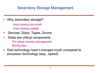
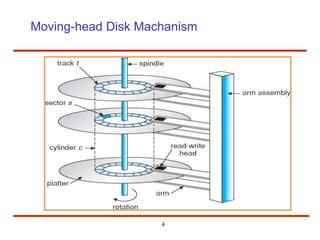
Disk Management refers to the process of managing and organizing computer storage devices, such as hard drives and solid-state drives. It involves tasks like creating partitions, formatting drives, assigning drive letters, and managing volumes. Disk Management is a critical aspect of maintaining and optimizing your computer's storage space.

1. 1
Mass-Storage Structure

2. Secendory Storage Management
• Why secondary storage?
main memory too small
main memory volatile
• Devices: Disks, Tapes, Drums
• Disks are critical components
For virtual memory management
Storing files
• Disk technology hasn’t changed much compared to
processor technology (esp., speed)
2

3. 3
Outline
• Disk Structure
• Disk Scheduling
• Disk Management
• Swap-Space Management
• RAID Structure
• Disk Attachment
• Stable-Storage Implementation
• Tertiary Storage Devices

4. 4
Moving-head Disk Machanism

5. 5
Overview of Mass Storage Structure
• Magnetic disks provide bulk of secondary storage of modern computers
– Drives rotate at 60 to 200 times per second
– Transfer rate is rate at which data flow between drive and computer
– Positioning time (random-access time) is time to move disk arm to
desired cylinder (seek time) and time for desired sector to rotate under the
disk head (rotational latency)
– Head crash results from disk head making contact with the disk surface
• That’s bad
• Disks can be removable
• Drive attached to computer via I/O bus
– Busses vary, including EIDE, ATA, SATA, USB, Fibre Channel, SCSI
– Host controller in computer uses bus to talk to disk controller built into
drive or storage array

6. 6
Disk Structure
• Disk drives are addressed as large 1-dimensional arrays of
logical blocks, where the logical block is the smallest unit of
transfer.
• The 1-dimensional array of logical blocks is mapped into the
sectors of the disk sequentially.
– Sector 0 is the first sector of the first track on the outermost cylinder.
– Mapping proceeds  (Cylinder, Track, Sector)
• In practice, not always possible
– Defective Sectors
– # of tracks per cylinders is not a constant

7. 7
Disk Scheduling

8. 8
Overview
• OS is responsible for using hardware efficiently
– For disk drives  fast access time and disk bandwidth
• Access time has two major components
– Seek time is the time for the disk to move the heads to the cylinder
containing the desired sector
• Seek time  seek distance
• Minimize seek time
– Rotational latency is the additional time waiting for the disk to rotate the
desired sector to the disk head
• Difficult for OS
• Disk bandwidth is the total number of bytes transferred, divided by the
total time between the first request for service and the completion of the
last transfer

9. 9
Overview (Cont.)
• Several algorithms exist to schedule the servicing of disk I/O
requests.
• We illustrate them with a request queue (0-199).
– 98, 183, 37, 122, 14, 124, 65, 67
– Head pointer 53

10. 10
FCFS
Illustration shows total head movement of 640 cylinders.

11. 11
FCFS
• Advantage
– Easy to understand and implement (queue)
– No Starvation (many suffer from convey effect)
– Can be used with less load
• Disadvantage
– Require more Seek time
– More waiting time and response time
– Inefficient

12. 12
SSTF
• Shortest-Seek-Time First (SSTF)
• Selects the request with the minimum seek time from the
current head position.
• SSTF scheduling is a form of SJF scheduling; may cause
starvation of some requests.
– Remember that requests may arrive at any time
• Not always optimal (how about 53371465…)

13. 13
SSTF (Cont.)
Illustration shows total head movement of 236 cylinders.

14. 14
SSTF (Cont.)
• Advantage
– Very efficientt in seek moves
– Increased throughput
Disadvantage
– Overhead to find out closest request
– Request far from head, will starve
– High variance in waiting time and response time

15. 15
SCAN
• The disk arm starts at one end of the disk, and moves
toward the other end, servicing requests until it gets to the
other end of the disk, where the head movement is reversed
and servicing continues.
• Sometimes called the elevator algorithm.

16. 16
SCAN (Cont.)
Say Head movement direction is towards 0
Illustration shows total head movement of 236 cylinders.

17. 17
SCAN (Cont.)
• Advantage
– Simple easy to understand and implement
– No Starvation (bounded waiting time)
Disadvantage
– Unnecessary mobile time till the end of the disk, even there is no request
– Longer waiting time for requesting just visited by head

18. 18
C-SCAN
• Provides a more uniform wait time than SCAN.
• The head moves from one end of the disk to the other,
servicing requests as it goes. When it reaches the other
end, however, it immediately returns to the beginning of the
disk, without servicing any requests on the return trip.
• Treats the cylinders as a circular list that wraps around from
the last cylinder to the first one.

19. 19
C-SCAN (Cont.)
Say Head movement direction is towards 199

20. 20
C-SCAN (Cont.)
• Advantage
– Provide uniform waiting time
– Better response time
• Disadvantage
– More seek movements compare to simple SCAN.

21. 21
LOOK Scheduling
• Look Scheduling
• Similar with Scan scheduling, but the disk arm only goes as
far as the final request in each direction
• For example, a disk queue with requests for I/O to sectors
on cylinders

22. 22
C-LOOK
• Version of C-SCAN
• Arm only goes as far as the last request in each direction,
then reverses direction immediately, without first going all
the way to the end of the disk.

23. 23
C-LOOK (Cont.)

24. 24
Selecting a Disk-Scheduling Algorithm
• SSTF is common and has a natural appeal
• SCAN and C-SCAN perform better for systems that place a heavy load
on the disk
– Remove starvation problem
• Performance relies on the number and types of requests
• Requests for disk service can be influenced by the file-allocation method
(Contiguous? Linked or Indexed?)
• Directory location and index blocks positions
– separate module of Disk Scheduling in the operating system,
• replaceable
• Either SSTF or LOOK is a reasonable choice for the default algorithm
• Scheduled by OS? Scheduled by disk controller?

25. 25
Disk Management

26. 26
Disk Formatting
• Typical sector is 512 bytes
 Preamble identifying start code and sector address
 Data
 Error correction code (16 bits). At least detecting errors possible
with probability almost 1
• Cylinder skew:
 After reading an entire track, as head is moved across a cylinder,
seeking next sector shouldn’t cause waiting for full rotation
• Interleaving sectors:
 As a sector is copied into controller buffer, it needs to be copied into
main memory. So next sector should not be adjacent if we wish to
avoid waiting for one full rotation

27. 27
Disk Partition
• To use a disk to hold files, OS still needs to record its own
data structures on the disk. it does so in two steps
• Partition the disk into one or more groups of cylinders
– Each partition can be treated as a separate disk
After partitioning , the second step is:
• Logical formatting or “making a file system”
– Store the initial file-system data structure onto the disk:
• Maps of free and allocated space (FAT or inode)
• Initial empty directory

28. 28
A Typical File-System Organization

29. 29
Boot Block
• Boot block initializes system
– Initialize CPU registers, device controllers, main memory
– Start OS
• A tiny bootstrap loader is stored in boot ROM
– Bring a full bootstrap program from disk
• Full bootstrap program is stored in boot blocks (fixed
location)
• The boot ROM instructs the disk controller to read the boot
blocks into memory, and then start executing the code to
load the entire OS

30. 30
MS-DOS Disk Layout

31. 31
Bad Blocks
• IDE
– MS-DOS format : write a special value into the corresponding FAT
entry for bad blocks
– MS-DOS chkdsk : search and lock bad blocks

32. 32
Bad Blocks – SCSI(Small Computer System Interface)
(Cont.)
• Controller maintains a list of bad blocks on the disk
• Low-level formatting  spare sectors (OS don’t know)
• Controller replaces each bad sector logically with one of the
spare sectors (sector sparing, or forwarding)
– Invalidate optimization by OS’s disk scheduling
– Each cylinder has a few spare sectors

33. 33
Bad Blocks – SCSI (Cont.)
• Typical bad-sector transaction
– OS tries to read logical block 87
– Controller calculates ECC and finds that it is bad. Report to OS
– Reboot next time, a special command is run to tell the controller to
replace the bad sector with a spare.
– Whenever the system requests block 87, it is translated into the
replacement sector’s address by the controller
• Sector slipping:
– Ex. Let sector 17 defective and first spare follows sector 202
• Spare  202  201  … 18  17

34. Read Errors
• After reading a sector, what if ECC indicates an error
– ECC may allow error correction
– Read again, and error may go away
– If read error seems to happen repeatedly, then the sector can be
marked as bad, and replaced by a spare sector
•Instead of the driver, OS may need to keep track of bad
sectors
•Backups have to worry about bad sectors
34

35. Reliability by Redundancy
• Mirroring (or Shadowing): duplicate disks
• Write every block to both the disks
• Read can be performed from any of the two disks
– This can be exploited to allow parallelism and speeding up of
reads
– Also for error correction: if first read fails, try the other
• Crash: If one disk crashes, then the other one can be
used to restore data
• If failures are independent, this dramatically increases
mean- time to failure
• This can be managed by device driver (if it can handle
multiple disks) or by OS
• Duplicating a disk is expensive.
35

36. RAID
Redundant Array of Independent Disks
• RAID (redundant array of independent disks) is a way of
storing the same data in different places on multiple hard
disks or solid-state drives to protect data in the case of a
drive failure. There are different RAID levels, however,
and not all have the goal of providing redundancy.
• Disk access times are still slow compared to
CPU/memory
• Natural solution: Read concurrently from multiple disks
• RAID Controller talks to OS just like a device driver and
manages a suite of disks to improve reliability and
performance
36

37. Key evaluation points for a RAID System
• Reliability: How many disk faults can the system tolerate?
• Availability: What fraction of the total session time is a
system in uptime mode, i.e. how available is the system for
actual use?
• Performance: How good is the response time? How high is
the throughput (rate of processing work)? Note that
performance contains a lot of parameters and not just the
two.
• Capacity: Given a set of N disks each with B blocks, how
much useful capacity is available to the user?
37

38. RAID levels
• Raid devices will make use of different versions, called
levels. The original paper that coined the term and
developed the RAID setup concept defined six levels of
RAID -- 0 through 5. This numbered system enabled those
in IT to differentiate RAID versions. The number of levels
has since expanded and has been broken into three
categories: standard, nested and nonstandard RAID levels.
38

39. RAID 0
• Array of disks with block-level striping
• Strip = k sectors (for suitably chosen k)
• First k sectors are on first strip of first disk, next k sectors are on
first strip of second disk, and so on
• Advantages:
– A large request spanning multiple strips can be parallelized easily
– Not much overhead
– Used in high-performance applications
• Disadvantages
– No redundancy
– Mean-time to failure is, in fact, less than standard disks (why?)
– No parallelism for small requests
39

40. RAID 0
40

41. RAID 1
41
• Like mirroring, but with striping of level 0
• Use same number of backup disks with same striping
• Same benefits/issues as in mirroring

42. RAID 2
42
 Called memory-style error correcting code organization
 Uses bit-level striping
 Some of the bits used for parity or other error correction
 Sample: 4-bits of data encoded by additional 3-bits of ECC, and
resulting 7 bits stored on 7 different disks
 CM-2 machine: 32-bits of data with 7-bits of ECC spanning over array of
39 disks
 Advantages
– Great parallelism for read as well as write
– Even if one disk crashes, all data can be recovered (due to ECC)
 Disadvantages
– Drives have to synchronized
– Overhead in putting together reads from different disks
– Crash recovery much slower (compared to RAID-1)

43. RAID 2
43

44. RAID 3
44
• This technique uses striping and dedicates one drive to
storing parity information.
• The embedded ECC information is used to detect errors.
• Data Recovery is accomplished by calculating the exclusive
information recorded on the other drives.
• Advantage
– Best for single-user systems with long record applications.
• Disadvantage
– Since an I/O operation addresses all the drives at the same time, RAID 3
cannot overlap I/O.

45. RAID 3
45

46. RAID 4
46
• This level uses large stripes.
• User can read records from any single drive.
• Overlapped I/O can then be used for read operations.
• Since all write operations are required to update the parity drive, no I/O
overlapping is possible.

47. RAID 5
47
• This level is based on parity block-level striping.
• The parity information is striped across each drive, enabling the array to
function even if one drive were to fail.
• Advantage
– The array's architecture allows read and write operations to span multiple
drives -- resulting in performance better than that of a single drive.
• Disadvantage
– Performance is not as high as that of a RAID 0 array.
– Considered to be a poor choice for use on write-intensive systems because
of the performance impact associated with writing parity data.
– When a disk fails, it can take a long time to rebuild a RAID 5 array.

48. RAID 5
48

49. Advantage of RAID
• An improvement in cost-effectiveness because lower-priced disks
are used in large numbers.
• The use of multiple hard drives enables RAID to improve on the
performance of a single hard drive.
• Increased computer speed and reliability after a crash --
depending on the configuration.
• Reads and writes can be performed faster than with a single drive
with RAID 0. This is because a file system is split up and
distributed across drives that work together on the same file.
• There is increased availability and resiliency with RAID 5. With
mirroring, RAID arrays can have two drives containing the same
data, ensuring one will continue to work if the other fails.
49

50. Disadvantage of RAID
• Nested RAID levels are more expensive to implement than
traditional RAID levels because they require a greater number of
disks.
• The cost per gigabyte of storage devices is higher for nested
RAID because many of the drives are used for redundancy.
• When a drive fails, the probability that another drive in the array
will also soon fail rises, which would likely result in data loss.
• Some RAID levels (such as RAID 1 and 5) can only sustain a
single drive failure.
• RAID arrays, and the data in them, are in a vulnerable state until
a failed drive is replaced and the new disk is populated with data.
50

51. Swap-space Management

52. Swap-Space Use
• Part of memory used as virtual memory space
• More swap memory reserved, may waste the
memory
• Less swap space may abort a process
• In Linux normally swap pace was kept double of the
physical memory, but now days it is a topic of
debate in Linux community
52

53. Swap-Space Location
• A swap space can reside in one of two locations:
– As a normal file system
• easy, but inefficient (time consuming)
• External fragmentation
– In a separate disk partition
• Swap space storage manager is used to allocate and deallocate
the memory
• Designed to improve speed rather storage
• internal fragmentation
– Mixed scheme
53