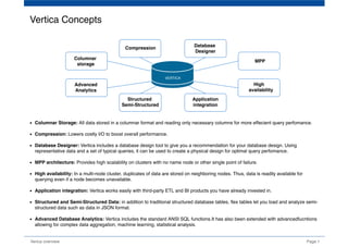
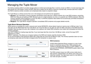
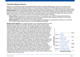
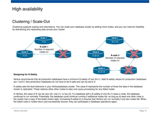
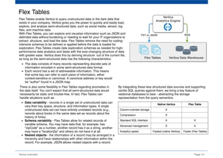
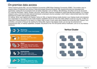
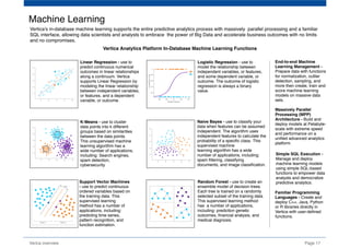
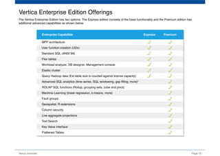
The document provides an overview of Vertica, a columnar storage database known for its efficient query performance through compression and optimized data storage. It highlights the architecture features such as MPP (massively parallel processing), high availability with data duplicates across nodes, and the use of flex tables for structured and semi-structured data. Additionally, it details the database design tool that aids users in optimizing their database schema and layout for improved analytics and storage efficiency.

1. Vertica quick overview
October 10, 2018
A.Sidelev

2. Vertica Concepts
Columnar
storage
Database
Designer
MPP
Application
integration
High
availability
Structured
Semi-Structured
Advanced
Analytics
Columnar Storage: All data stored in a columnar format and reading only necessary columns for more effecient query perfomance.
Compression: Lowers costly I/O to boost overall performance.
Database Designer: Vertica includes a database design tool to give you a recommendation for your database design. Using
representative data and a set of typical queries, it can be used to create a physical design for optimal query perfomance.
MPP architecture: Provides high scalability on clusters with no name node or other single point of failure.
High availability: In a multi-node cluster, duplicates of data are stored on neighboring nodes. Thus, data is readily available for
querying even if a node becomes unavailable.
Application integration: Vertica works easily with third-party ETL and BI products you have already invested in.
Structured and Semi-Structured Data: in addition to traditional structured database tables, flex tables let you load and analyze semi-
structured data such as data in JSON format.
Advanced Database Analytics: Vertica includes the standard ANSI SQL functions.It has also been extended with advancedfucntions
allowing for complex data aggregation, machine learning, statistical analysis.
Page 1Verica overview
Compression
VERTICA

3. Unsorted data
string
BBBBCCCC
CCCCAAAA
...
AAAABBBB
...
SELECT MAX(number) FROM table WHERE date = '2018-09-01' AND string = 'AAAABBBB';
Sorted data
number date
22222222
33333333
...
55555555
...
2001-12-31
2018-09-01
...
2018-10-05
...
string
AAAABBBB
BBBBCCCC
...
CCCCAAAA
...
Verica overview Page 2
Columnar storage
In traditional row-store databases, data is stored in tables. Vertica
organizes data in subsets of columns, called - projections.
When a query is submitted to a traditional row-store database, every
column in the table is examined in order t provide the query response.
In Vertica, only the columnsreferenced in the query statement are
examined; the significant reduction in disk I/O and storage space allows
for much faster query perfomance and response.
Vertica stores data in a column format so it can be queried for best
performance. Compared to row-based storage, column storage reduces
disk I/O making it ideal for read-intensive workloads. Vertica reads only
the columns needed to answer the query.
...
...
...
...
...
...
...
...
...
...
...
...
...
...
...
...
...
...
...
...
number date
55555555
22222222
...
33333333
...
2018-09-01
2018-10-05
...
2017-12-31
...
. . . . .
.....
Columnar StorageRow Storage
Traditional Database
Storage Method
Requires all data be read
on query
Limited compression
possible
Vertica Database Storage
Method
Speeds Query Time by
Reading Only Necessary
Data
Ready for Compression

4. Page 3Verica overview
Projection hierarchy in the Database
TABLES
PROJECTIONS
PROJECTION_COLUMNS
PROJECTION_STORAGE
Vertica object hierarchy
A B C
A B C A BC AC
A1.gt
B1.gt
C1.gt
A2.gt
B2.gt
C2.gt
A3.gt
B3.gt
C3.gt
A4.gt
B4.gt
C4.gt
users
users_p1 users_p2 users_p3
Table
(logical)
Projections
(physical)
Containers
Files
In order to allow the use of ANSI SQL commands (SELECT/INSERT/DELETE), we reference information based on the table name. The
tables are maintained as virtual object; data is not stored in them.
Each table is used as the basic for one or more physical projections; the projections contain subsets of the column in the table. Data is
arranged in the projections; each projection column is sorted and encoded/compressed based on the type of data in the column.
Queries run against data stored in this format run more quickly than against row-store storage.
All data is stored on disk encoded/comressed, and is organized is ROS comntainers. While the maximum number of containers pre
projection is 1024, recommend thenubber around 700.
Each time data is inserted into the projection, it is stored on disk in compressed .gt files in the /data directory.

5. Page 4Verica overview
Encoding converts data into a standard format and increases performance because there is less disk I/O during query execution. It also
passes encoded values to other operations, saving memory bandwidth. Vertica uses several encoding strategies, depending on data type,
table cardinality, and sort order. Vertica can directly process encoded data. Run the Database Designer for optimal encoding in your
physical schema. The Database Designer analyzes the data in each column and recommends encoding types for each column in the
proposed projections, depending on your design optimization objective. For flex tables, Database Designer recommends the best encoding
types for any materialized flex table columns, but not for __raw__ column projections.
Encoding type Data type Cardinality Sorted
BLOCK_DICT
CHAR(short)
VARCHAR(short)
LOW No
DELTARANGE_COMP FLOAT HIGH Yes
DELTAVAL
INTEGER
DATE
TIME
TIMESTAMP
INTERVAL
HIGH Yes
RLE
CHAR
VARCHAR
NUMERIC
LOW Yes
Data encoding
BLOCK_DICT - For each block of storage, Vertica compiles distinct column values into a dictionary and then stores the dictionary and a
list of indexes to represent the data block. BLOCK_DICT is ideal for few-valued, unsorted columnswhere saving space is more important
than encoding speed. Certain kinds of data, such as stock prices, are typically few-valued within a localized area after the data is sorted,
such as by stock symbol and timestamp, and are good candidates for BLOCK_DICT. BLOCK_DICT encoding requires significantly higher
CPU usage than default encoding schemes. The maximum data expansion is eight percent (8%).
DELTARANGE_COMP - This compression scheme is primarily used for floating-point data; it stores each value as a delta from the
previous one. This scheme is ideal for many-valued FLOAT columns that are sorted or confined to a range. This scheme has a high cost
for both compression and decompression.
DELTAVAL - For INTEGER and DATE/TIME/TIMESTAMP/INTERVAL columns, data is recorded as a difference from the smallest value in
the data block. This encoding has no effect on other data types. DELTAVAL is best used for many-valued, unsorted integer or integer-
based columns. CPU requirements for this encoding type are minimal, and data never expands.
RLE - RLE (run length encoding) replaces sequences (runs) of identical values with a single pair that contains the value and number of
occurrences. Therefore, it is best used for low cardinality columns that are present in the ORDER BY clause of a projection. The Vertica
execution engine processes RLE encoding run-by-run and the Vertica optimizer gives it preference. Use it only when run length is large,
such as when low-cardinality columns are sorted. The storage for RLE and AUTO encoding of CHAR/VARCHAR and
BINARY/VARBINARY is always the same.

6. Data compression
Compression transforms data into a compact format. Vertica uses integer packing for unencoded integers and LZO for compressed data.
Before Vertica can process compressed data it must be decompressed. Compression allows a column store to occupy substantially less
storage than a row store. In a column store, every value stored in a column of a projection has the same data type. This greatly facilitates
compression, particularly in sorted columns. In a row store, each value of a row can have a different data type, resulting in a much less
effective use of compression. Vertica compresses flex table __raw__ column data by about one half (1/2). The efficient storage methods
that Vertica uses for your database allows you to you maintain more historical data in physical storage.
Page 5Verica overview
Compression type Data type Cardinality Sorted
Lempel-Ziv-Oberhumer (LZO)
Compiles and indexes distinct column values
BINARY
VARBINARY
BOOLEAN
CHAR
VARCHAR
FLOAT
HIGH No
Compression scheme based on the delta
between consecutive column values
DATE
TIME
TIMESTAMP
INTEGER
INTERVAL
HIGH No
LZO - LZO (Lempel-Ziv-Oberhumer) is a lossless data compression algorithm that is focused on decompression speed with characteristics:
compression comparable in speed to DEFLATE compression
very fast decompression
requires an additional buffer during compression (of size 8 kB or 64 kB, depending on compression level)
requires no additional memory for decompression other than the source and destination buffers
allows the user to adjust the balance between compression ratio and compression speed, without affecting the speed of decompression
LZO supports overlapping compression and in-place decompression. As a block compression algorithm, it compresses and
decompresses blocks of data. Block size must be the same for compression and decompression. LZO compresses a block of data into
matches (a sliding dictionary) and runs of non-matching literals to produce good results on highly redundant data and deals acceptably
with non-compressible data, only expanding incompressible data by a maximum of 1/64 of the original size when measured over a block
size of at least 1 kB.
DELTAVAL - For INTEGER and DATE/TIME/TIMESTAMP/INTERVAL columns, data is recorded as a difference from the smallest value in
the data block. This encoding has no effect on other data types. DELTAVAL is best used for many-valued, unsorted integer or integer-
based columns. CPU requirements for this encoding type are minimal, and data never expands.
GCDDELTA - For INTEGER and DATE/TIME/TIMESTAMP/INTERVAL columns, and NUMERIC columns with 18 or fewer digits, data is
recorded as the difference from the smallest value in the data block divided by the greatest common divisor (GCD) of all entries in the
block. This encoding has no effect on other data types. ENCODING GCDDELTA is best used for many-valued, unsorted, integer columns
or integer-based columns, when the values are a multiple of a common factor. The CPU requirements for decoding GCDDELTA encoding
are minimal, and the data never expands, but GCDDELTA may take more encoding time than DELTAVAL.

7. DESIGNER_SET_DESIGN_TYPE - types of projections is comprehensive or incremental.
- comprehensive (default) creates an initial or replacement design for all tables in the specified schemas. You typically create
a comprehensive design for a new database.
- incremental modifies an existing design with additional projection that are optimized for new or modified queries.
DESIGNER_SET_DESIGN_KSAFETY - sets K-safety for a comprehensive design and stores the K-safety value in the DESIGNS table.
Database Designer ignores this function for incremental designs.
- k‑level an integer between 0 and 2 that specifies the level of K-safety for the target design. This value must be compatible with the number
of nodes in the database cluster:
k‑level = 0: ≥ 1 nodes
k‑level = 1: ≥ 3 nodes
k‑level = 2: ≥ 5 nodes
DESIGNER_SET_OPTIMIZATION_OBJECTIVE - specifies whether the design optimizes for query or load performance. Valid only for
comprehensive database designs, specifies the optimization objective Database Designer uses. Database Designer ignores this function for
incremental designs.
- QUERY: Optimize for query performance. This can result in a larger database storage footprint because additional projections might be
created.
- LOAD: Optimize for load performance so database size is minimized. This can result in slower query performance.
- BALANCED (default): Balance the design between query performance and database size.
DESIGNER_SET_PROPOSE_UNSEGMENTED_PROJECTIONS - Enables inclusion of unsegmented projections in the design.
DESIGNER_SET_ANALYZE_CORRELATIONS_MODE - Determines how the design handles column correlations.
Verica overview Page 6
Automatic Database Design
Vertica includes the Database Designer (DBD), a tool that minimizes DBA's burden of optimizing the database for query perfomanceand
and data loading. While the use of the tool is not required, considerable perfomance benefits can be achieved by implementing its
recomendations.
User provides BenefitsDatabase designer
Logical Schema
Sample Data
Tupical Queries
Design Goals
Lower Hardware Costs
Faster Queries
Optimize Perfomance
Optimize Load and
Storage Data
Data Encoding
Data Compression
Design main properties:

8. Page 7Verica overview
To support loading data into the database, intermixed with ueries in a typical data warehouse workload, Vertica implements the storage
model shown in theillustration below. This model is the same on each Vertica node.
The Write Optimized Store (WOS) is a memory-resident data store. Temporarilly storing data in memory speeds up the loading process
and reduces fragmentation on disk; the data is still available for queries. For organizations who continually load small amounts of data,
loading the data to memory first is faster than writing it to disk, making the data accessible quikly.
The Read Optimized Store (ROS) is a disk resident data store. When the Tuple Mover task moveout is run, containers are created in the
ROS and the data is organized in projections on disk.
Both the WOS and the ROS exist on each node in the cluster.
The Hybrid Storage Model
Write Optimized Store
(WOS)
Read Optimized Store
(ROS)
In memory
Unencode
Unsorted
Uncompressed
Segmented
K-safe
Low latency / small quick
A
A1
A2
B
B1
B2
C
C1
C2
On disk
Encode
Sorted
Compressed
Segmented
K-safe
Large data loaded
directly
TUPLE MOVER
moveout
mergeout
The Tuple Mover moves data from the WOS (memory) to the ROS (disk) using the
following processes:
Moveout copies data from the WOS to the Tuple Mover and then to the ROS; data is sorted, encoded, and compressed into files.
Mergeout combines smaller ROS containers into larger ones to reduce fragmentation.
The Tuple Mover automatically performs these tasks in the background, at intervals that are set by its configuration parameters.
Each of these operations occurs at different intervals across all nodes. The Tuple Mover runs independently on each node, ensuring that
storage is managed appropriately even in the event of data skew.
You usually use the COPY statement to bulk load data. It can load data into WOS, or load data directly into the ROS.
MEMORY DISK

9. Page 8Verica overview
Managing the Tuple Mover
The Vertica analytics platform provides storage options to trickle load small data files in memory, known as WOS, or to bulk load large data
files directly into a file system, known as ROS. Data that is loaded into the WOS is stored as unsorted data, whereas data that is loaded
into ROS is stored as sorted, encoded, and compressed data, based on projection design.
The Tuple Mover is a Vertica service that runs in the background and performs two operations:
Moveout: The Tuple Mover moveout operation periodically moves data from a WOS container into a new ROS container, preventing
WOS from filling up and spilling to ROS. Moveout runs on a single projection at a time, on a specific set of WOS containers. When the
moveout operation picks projections to move into ROS, it combines projection data loaded from all previously committed transactions
and writes them into a single ROS container.
Mergeout: The Tuple Mover mergeout operation consolidates ROS containers and purges deleted records.
Tuple Mover Moveout Operation
WOS memory is controlled by a built-in resource pool named WOSDATA, whose default maximum memory size is 2GB per node. If you
load data into the WOS faster than the Tuple Mover can move the data out, the data can spill into ROS until space in the WOS becomes
available. Data loss does not occur with a spillover, but a spillover can create ROS containers much faster than anticipated and slows the
moveout operation.
Use COPY DIRECT for loading large data files. If you load large data files (more than 100 MB per node), convert the large COPY
statement to a COPY
DIRECT statement. This allows you to bypass loading to the WOS and instead, load files directly to ROS.
Do not use the WOS to load temporary tables with a large data set (more than 50 MB per node). The moveout operation does not move
out temporary table data and the data is dropped when the transaction or session ends.
Time
Now
0 3
Time
Now
WOS
WOS
ROS container
MOVEOUT
ROS Containers
A ROS (Read Optimized Store) container is a set of rows
stored in a particular group of files. ROS containers are
created by operations like Moveout or COPY DIRECT. You
can query the STORAGE_CONTAINERS system table to see
ROS containers.
The ROS container layout can differ across nodes due to
data variance. Segmentation can deliver more rows to one
node than another. Two data loads could fit in the WOS on
one node and spill on another.

10. Tuple Mover Mergeout Operation
Mergeout is the Tuple Mover process that consolidates ROS containers and purges deleted records. Over time, the number of ROS
containers increases enough to affect performance. It is then necessary to merge some of the ROS containers to avoid performance
degradation. At that point, the Tuple Mover performs an automatic mergeout, combining two or more ROS containers into a single container.
Partition Mergeout. Vertica keeps data from different table partitions or partition groups separate on disk. The Tuple Mover adheres to this
separation policy when it consolidates ROS containers. When a partition is first created, it typically has frequent data loads and requires
regular activity from the Tuple Mover. As a partition ages, it commonly transitions to a mostly read-only workload and requires much less
activity. The Tuple Mover has two different policies for managing these different partition workloads:
Active partition is the partition that was most recently created. The Tuple Mover uses a STRATA mergeout policy that keeps a
collection of ROS container sizes to minimize the number of times any individual tuple is subjected to mergeout. A table's active
partition count identifies how many partitions are active for that table.
Inactive partitions are those that were not most recently created. The Tuple Mover consolidates ROS containers to a minimal set
while avoiding merging containers whose size exceeds MaxMrgOutROSSizeMB.
Mergeout Strata Algorithm. The mergeout operation uses a strata-based algorithm to verify
that each tuple is subjected to a mergeout operation a small, constant number of times,
despite the process used to load the data. The mergeout operation uses this algorithm to
choose which ROS containers to merge for non-partitioned tables and for active partitions in
partitioned tables. Vertica builds strata for each active partition and for projections anchored
to non-partitoned tables. The number of strata, the size of each stratum, and the maximum
number of ROS containers in a stratum is computed based on disk size, memory, and the
number of columns in a projection. Merging small ROS containers before merging larger
ones provides the maximum benefit during the mergeout process. The algorithm begins at
stratum 0 and moves upward. It checks to see if the number of ROS containers in a stratum
has reached a value equal to or greater than the maximum ROS containers allowed per
stratum. The default value is 32. If the algorithm finds that a stratum is full, it marks the
projections and the stratum as eligible for mergeout. The mergeout operation combines ROS
containers from full strata and produces a new ROS container that is usually assigned to the
next stratum. With the exception of stratum 0, the mergeout operation merges only those
ROS containers equal to the value of ROSPerStratum. For stratum 0, the mergeout
operation merges all eligible ROS containers present within the stratum into one ROS
container. By default, the mergeout operation has two threads. Typically, the mergeout of
large ROS containers in higher stratum takes longer than the mergeout of ROS containers in
lower stratum. Only mergeout thread 0 can work on higher stratum and inactive partitions.
This restriction prevents the accumulation of ROS containers in lower stratum, because
mergeout thread 0 takes more time to perform mergeouts in higher stratum. Mergeout thread
1 operates only on the lower strata.
Page 9Verica overview
64MB
64GB
16GB
4GB
256MB
Stratum 0
Stratum 1
Stratum 2
Stratum 3
Stratum 4
Start Epoch, End Epoch
ROSContainerSize

11. Page 10Verica overview
Loading Data
If you have small, frequent data loads (trickle loads), best practice is to load the records into memory, into the WOS. Data loaded to the
WOS is still available for query results. The size of the WOS is limited to 25% of the availeble RAM or 2GB, whichever is smaller. If the
amount of data loaded to WOS exceeds this size, the data is automatically spilled to disk in the ROS.
For the initial data load, and for subsequent large loads, best practice is to load the data directly to disk where it will be stored in the ROS.
This process leads to the most efficient loading with the least demand on cluster resources.
Write Optimized Store
(WOS)
Read Optimized Store
(ROS)
Trickle Load
COPY
INSERT
UPDATE
DELETE
Bulk Load
COPY DIRECT
INSERT /*+ DIRECT */
UPDATE /*+ DIRECT */
DELETE /*+ DIRECT */
automatic spillover
INSERT vs. COPY to Load Data
Insert one row of data at a time
Record-by-record resource cost
Use for small, infrequent loads
Bulk load of data
Resource overhead cost paid once
Use for large loads
Large files can be split for parallel
loads
INSERT COPY
Choosing a Load Method
This is the default load method. If you do not specify a load
option explicitly, COPY uses the AUTO method to load data
into WOS (Write Optimized Store) in memory. The default
method is good for smaller bulk loads (< 100MB). Once the
WOS is full, COPY continues loading directly to ROS (Read
Optimized Store) on disk. ROS data is sorted and encoded.
Use the DIRECT parameter to to load data directly into ROS
containers, bypassing loading data into WOS. The DIRECT
option is best suited for large data loads (100MB or more).
Using DIRECT to load many smaller data sets results in many
ROS containers, which have to be combined later.
Use the TRICKLE option to load data incrementally after you
complete your initial bulk load. Trickle loading loads data into
the WOS. If the WOS becomes full, an error occurs and the
entire data load is rolled back. Use this option only when you
have a finely-tuned load and moveout process at your site, and
you are confident that the WOS can hold the data you are
loading. This option is more efficient than AUTO when loading
data into partitioned tables.
By default, COPY uses the DELIMITER parser to load raw data
into the database. Raw input data must be in UTF-8, delimited
text format. COPY parsers include:
DELIMITED | NATIVE BINARY | NATIVE VARCHAR | FIXED-
WIDTH | ORC | PARQUET
AUTO
DIRECT
TRICKLE
COPY
PARSERS
Vertica Transaction Model
time
Closed Epoch Current Epoch
Ancient History Mark
(AHM)
Historical
Epochs
(no locks)
Latest
Epoch
(no locks)
Current
Epoch
advanced on
DML commit
INSERTS,
DELETES,
or
UPDATES
AHM: The Ancient History Mark epoch prior to which
historical data can be purged from physical storage.
Epoch: A 64-bit number representing a logical
timestamp for data in Vertica. Every row has an
implicitly stored column recording the committed epoch.
The epoch advances when the logical state of the
system changes or when data is committed with
DML operations (INSERT, UPDATE, MERGE,
COPY, or DELETE).

12. MassivelyParallelProcessing
Verica overview Page 11
MPP database is a type of database or data warehouse where the data and processing power are split up among several different nodes
(servers), with one leader node and one or many compute nodes. MPP databases can scale horizontally by adding more compute
resources (nodes), rather than having to worry about upgrading to more and more expensive individual servers (scaling vertically). Adding
more nodes to a cluster allows the data and processing to be spread across more machines, which means the query will be completed
sooner.
Without this structure, running even the simplest of queries on large dataset would take a prohibitively long time.
Parallel design
Enables distributed storage and workload with active redundancy
Automatic replication, failover and recovery
Shared-nothing database architecture
Provides high scalability on clusters
No name node or other single point of failure
Add nodes to achieve optimal capacity and performance
Lower data center costs, higher density, scale-out
Distributed query execution
1. Client connects to a node and issues a query
- Node the client is connected to becomes the initiator node
- Other nodes in the cluster become executor nodes
2. Initiator node parses the query and picks an execution plan
3. Initiator node distributes query plan to executor nodes
4. Initiator node aggregates results from all nodes
5. Initiator node returns final result to the user
Any node can be the initiator
No name node or single point of failure
Query/Load to any node
Continuous/real-time load and query
Nodes are Peers
private network
proxy balancer
public network
INITIATOREXECUTOR EXECUTOR
CPU * RAM * DISK CPU * RAM * DISK CPU * RAM * DISK

13. High availability
Verica overview Page 12
Clustering / Scale-Out
Clustering supports scaling and redundancy. You can scale your database cluster by adding more nodes, and you can improve reliability
by distributing and replicating data across your cluster.
1 | 2
2 | 31 | 3
Node 1
Node 2Node 3
5 | 1 | 2
1 | 2 | 31 | 5 | 4
Node 1
Node 2Node 5
5 | 4 | 3
Node 4
2 | 3 | 4
Node 3
K-safe 1
Number of required
nodes 3+
K-safe 2
Number of required
nodes 5+
Designing for K-Safety
Vertica recommends that all production databases have a minimum K-safety of one (K=1). Valid K-safety values for production databases
are 1 and 2. Non-production databases do not have to be K-safe and can be set to 0.
K-safety sets the fault tolerance in your Verticadatabase cluster. The value K represents the number of times the data in the database
cluster is replicated. These replicas allow other nodes to take over query processing for any failed nodes.
In Vertica, the value of K can be zero (0), one (1), or two (2). If a database with a K-safety of one (K=1) loses a node, the database
continues to run normally. Potentially, the database could continue running if additional nodes fail, as long as at least one other node in
the cluster has a copy of the failed node's data. Increasing K-safety to 2 ensures that Vertica can run normally if any two nodes fail. When
the failed node or nodes return and successfully recover, they can participate in database operations again.

14. Verica overview Page 13
INFRASTRUCTURE
CLOUD
ADVANCED
ANALYTICS
HADOOP
VERTICA
DATA INTEGRATIONBI / VISUALISATION
Application integration

15. Page 14Verica overview
Flex Tables
Flex Tables enable Vertica to query unstructured data or the dark data that
exists in your company. Vertica gives you the power to quickly and easily load,
explore, and analyze semi-structured data, such as social media, sensor, log
files, and machine data.
With Flex Tables, you can explore and visualize information such as JSON and
delimited data without burdening or needing to wait for your IT organizations to
extract, structure, and load the data. Flex Tables remove the need for coding-
intensive schemas to be defined or applied before the data is loaded for
exploration. Flex Tables create data exploration schemas as needed for high-
performance data analytics and deals with the ever-changing structure of data
with greater ease. Vertica does this by deriving structure out of the current file,
as long as the semi-structured data has the following characteristics: Vertica Data WarehouseFlex Tables
Vertica
Analytics Engine
The data consists of many records representing discrete sets of
information encoded in some semi-structured data format.
Each record has a set of addressable information. This means
that some key can refer to each piece of information, either
context-sensitive or canonical. A canonical address or key would
be "author" found in a JSON map.
There is also some flexibility in Flex Tables regarding anomalies in
the data itself. You can't expect that all semi-structured data would
necessarily be static and trouble-free. In fact, Flex Tables can
handle situations such as:
Data variability - records in a single set of unstructured data can
vary their key space, structure, and information types. A single
unstructured data set can have entirely unrelated records (e.g.,
records about books in the same data set as records about the
history of forks).
Schema variability - Flex Tables allow for related records of
variable schema. You may have data that, for example, has
"zipCode" as a number, another record has it as a string, another
may have a "locationZip" and others do not have it at all.
Nested objects - the information of a record may be arranged in a
hierarchy and have relationships with other information within the
record. For example, JSON allows nested objects with a record.
By integrating these less structured data sources and supporting
vanilla SQL queries against them, we bring a key feature of
relational databases to bear - abstracting the storage
representation from the query semantics.
TXT or JSON ROS
Native Vertica Flex Table
Column-oriented storage X
Compression X
Standard SQL interface X X
Advanced management X X
Analytics speed Fastest (native Vertica) Faster (Flex Tables)

16. Page 15Verica overview
Advanced In-database Analytics
SQL 99 In-database AnalyticsSDKsSQL Extensions
Aggregate
Analytical
Window functions
Graph
Monte Carlo
Statistical
Geospatial
Pattern matching
Event series joins
Time series
Event-based windows
Java
C++
R
ODBC/JDB
HIVE
Hadoop
Flex zone
Analytics Connection Regression testing
K-means
Statistical modeling
Classification
algorithms
Page rank
Text mining
Allows for:
standard functionality
thatperforms at scale
Allows for:
Sessionization
Conversion analysis
Fraud detection
Fast Aggregates (LAP)
Allows for:
Machine learning
Custom data mining
Specialized parsers
Allows for:
Statistical modeling
Cluster analysis
Predictive analytics

17. Page 16Verica overview
On-premise data access
Streaming
Kafka, Spark, Trickle (Insert/Update)
Schema on read
Flex Zone: JSON, CSV, TEXT,
Social Media.
Batch
ODBC/JDBC, Bulk COPY, LCOP,
ETL: Pentaho, Attunity, Informatica,
Talend, ET AL
Unstructured
IDOL: Video, Audio, Voice
Recognition, Facial Recognition
Hadoop
ORC Reader, MapR NFS, HIVE
Serializer: HDFS, Parquet, AVRO
Vertica Cluster
Vertica supports popular SQL, and Java Database Connectivity (JDBC)/Open Database Connectivity (ODBC). This enables users to
preserve years of investment and training in these technologies because all popular SQL programming tools and languages work
seamlessly. Leading BI and visualization tools are tightly integrated, such as Tableau, MicroStrategy, and others and so are all popular
ETL tools like Informatica, Talend, Pentaho, and more. Vertica offers maximum scalability for large-scale Big Data analytics. It is uniquely
designed using a memory-and-disk balanced distributed compressed columnar paradigm, which makes it exponentially faster than older
techniques for modern data analytics workloads.
On Hadoop: When used together with Hadoop, Vertica for SQL on Apache Hadoop installs directly in your Hadoop cluster and empowers
your organization to use a powerful set of data analytics capabilities and do far more than either platform could do on its own. It offers no
single point of failure because it's not reliant on a helper node to query. It even reads native Hadoop file formats like ORC, Parquet, Avro,
and others, and writes to Parquet. By installing the Vertica SQL engine in the Hadoop cluster, you can tap into advanced and
comprehensive SQL on Hadoop capabilities, complete 100 percent of the TPC-DS queries without modification, and run on any Hadoop
distribution.

18. Page 17Verica overview
Machine Learning
Vertica's in-database machine learning supports the entire predictive analytics process with massively parallel processing and a familiar
SQL interface, allowing data scientists and analysts to embrace the power of Big Data and accelerate business outcomes with no limits
and no compromises.
Linear Regression - use to
predict continuous numerical
outcomes in linear relationships
along a continuum. Vertica
supports Linear Regression by
modeling the linear relationship
between independent variables,
or features, and a dependent
variable, or outcome.
Logistic Regression - use to
model the relationship between
independent variables, or features,
and some dependent variable, or
outcome. The outcome of logistic
regression is always a binary
value.
K-Means - use to cluster
data points into k different
groups based on similarities
between the data points.
This unsupervised machine
learning algorithm has a
wide number of applications,
including: Search engines,
spam detection,
cybersecurity.
Naive Bayes - use to classify your
data when features can be assumed
independent. The algorithm uses
independent features to calculate the
probability of a specific class. This
supervised machine
learning algorithm has a wide
number of applications, including:
spam filtering, classifying
documents, and image classification.
Support Vector Machines
- use to predict continuous
ordered variables based on
the training data. This
supervised learning
method has a number of
applications, including:
predicting time series,
pattern recognition, and
function estimation.
Random Forest - use to create an
ensemble model of decision trees.
Each tree is trained on a randomly
selected subset of the training data.
This supervised learning method
has a number of applications,
including: prediction genetic
outcomes, financial analysis, and
medical diagnosis.
End-to-end Machine
Learning Management -
Prepare data with functions
for normalization, outlier
detection, sampling, and
more then create, train and
score machine learning
models on massive data
sets.
Massively Parallel
Processing (MPP)
Architecture - Build and
deploy models at Petabyte-
scale with extreme speed
and performance on a
unified advanced analytics
platform.
Simple SQL Execution -
Manage and deploy
machine learning models
using simple SQL-based
functions to empower data
analysts and democratize
predictive analytics.
Familiar Programming
Languages - Create and
deploy C++, Java, Python
or R libraries directly in
Vertica with user-defined
functions.
Vertica Analytics Platform In-Database Machine Learning Functions

19. External tables
(Flex tables)
COPY
Page 18Verica overview
Vertica for SQL on Apache Hadoop
Vertica SQL on Apache Hadoop offers the fastest and most enterprise-ready way to perform SQL queries on your Hadoop data. We’ve
leveraged our years of experience in the big data analytics marketplace and now offer the same technology that powers the Vertica
database to command a query engine for data stored in HDFS. Users can perform analytics regardless of the format of data or Hadoop
distribution used.
Vertica SQL on Apache Hadoop handles your mission-critical analytics projects by merging the best of our analytics platform with the best
that Hadoop data analytics can offer. The principles below help us to deliver on these promises:
Data lake or daily analytics. The SQL engine supports data discovery on your Hadoop data lake as well as highly optimized
analytics for even the most demanding SLAs.
Unified analytics engine. The engine is flexible enough to perform analytics on data no matter where it lives—Hadoop, native
Vertica, or in the cloud.
Complete SQL support. Get full ANSI SQL 99 compliance that is able to execute 100 percent of the TPC-DS benchmarks without
modification.
Workload management. Convenient, graphical application supports Ambari to check the health of both the Vertica and Hadoop
clusters and their queries. It also supports storage labels for resource allocation in YARN.
Fast ORC and Parquet file readers. Vertica can quickly and efficiently query ORC and Parquet files for fast Hadoop data analytics
without moving the data. Other formats like AVRO are also supported.
Clickstream, Web SessionDataArchived Data HDFS
VERTICA
/catalog
/data
Hive Pig
MapReduce
HBase
HCatalog
Archived Storage
Hive integration
(through HCatalog)
Read
Vertica can read structured information in
HCatalog, which reads directly from HDFS
Vertica includes the ability to read the Hive
data warehouse through HCatalog
Row-oriented data in Hadoop can be
streamed into Vertica external tables;
only the results of the query are stored in
these tables
The SQL COPY command can be used to
move data out of the Hadoop data lake for
storage in Vertica using the HDFS
Connectior
HDFS can act as an "infinite disk" for
Vertica, allowing unused or irregularly
accessed data to be stored outside of the
Vertica database
The following image summarizes the
different integration points between Vertica
and Hadoop:

20. Page 19Verica overview
Vertica Enterprise Edition Offerings
The Vertica Enterprise Edition has two options. The Express edition consists of the base functionality and the Premium edition has
additional advanced capabilities as shown below.
Enterprise Capabilitie Express Premium
MPP architecture
Workload analyzer, DB designer, Management console
Standard SQL (ANSI 99)
Flex tables
User function creation (UDx)
Elastic cluster
Machine Learning (linear regression, k-means, more)
Advanced SQL analytics (time series, SQL windowing, gap filling, more)*
ROLAP SQL functions (Rollup, grouping sets, cube and pivot)
Query Hadoop data (Ext table size is counted against license capacity)
Fault groups
Geospatial, R extensions
Column security
Live aggregate projections
Text Search
Key Value interface
Flattened Tables