
Recommended
More Related Content
Similar to SFG.pptx
Similar to SFG.pptx (20)
More from abbas miry
More from abbas miry (13)
Recently uploaded
Recently uploaded (20)
SFG.pptx
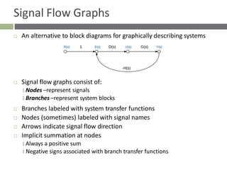
- 1. Signal Flow Graphs An alternative to block diagrams for graphically describing systems Signal flow graphs consist of: 🞑 Nodes –represent signals 🞑 Branches –represent system blocks Branches labeled with system transfer functions Nodes (sometimes) labeled with signal names Arrows indicate signal flow direction Implicit summation at nodes 🞑 Always a positive sum 🞑 Negative signs associated with branch transfer functions
- 2. Block Diagram → Signal Flow Graph Toconvert from a block diagram to a signal flow graph: 1. Identify and label all signals on the block diagram 2. Place a node for each signal 3. Connect nodes with branches in place of the blocks Maintain correct direction Label branches with corresponding transfer functions Negate transfer functions as necessary to provide negative feedback 4. If desired, simplify where possible
- 3. Signal Flow Graph – Example 1 Convert to a signal flow graph Label any unlabeled signals Place a node for each signal
- 4. Signal Flow Graph – Example 1 Connect nodes with branches, each representing a system block Note the -1 to provide negative feedback of X2 𝑠
- 5. Signal Flow Graph – Example 1 Nodes with a single input and single output can be eliminated, if desired 🞑 This makes sense for X1 𝑠 and X2 𝑠 🞑 Leave 𝑈 𝑠 to indicate separation between controller and plant
- 6. Signal Flow Graph – Example 2 Revisit the block diagram from earlier 🞑 Convert to a signal flow graph Label all signals, then place a node for each
- 7. Signal Flow Graph – Example 2 Connect nodes with branches
- 8. Signal Flow Graph – Example 2 Simplify – eliminate X5 𝑠 , X6 𝑠 , X7 𝑠 , and X8 𝑠
- 9. 40 Mason’s Rule We’ve seen how to reduce a complicated block diagram to a single input-to-output transfer function 🞑 Many successive simplifications Mason’s rule provides a formula to calculate the same overall transfer function 🞑 Single application of the formula 🞑 Can get complicated Before presenting the Mason’s rule formula, we need to define some terminology
- 10. 41 Loop Gain Loop gain – total gain (product of individual gains) around any path in the signal flow graph 🞑 Beginning and ending at the same node 🞑 Not passing through any node more than once Here, there are three loops with the following gains: 1. −𝐺1𝐻3 2. 𝐺2𝐻1 3. −𝐺2𝐺3𝐻2
- 11. 42 Forward Path Gain Forward path gain – gain along any path from the input to the output 🞑 Not passing through any node more than once Here, there are two forward paths with the following gains: 1. 𝐺1𝐺2𝐺3𝐺4 2. 𝐺1𝐺2𝐺5
- 12. 43 Non-Touching Loops Non-touching loops – loops that do not have any nodes in common Here, 1. −𝐺1𝐻3 does not touch 𝐺2𝐻1 2. −𝐺1𝐻3 does not touch −𝐺2𝐺3𝐻2
- 13. 44 Non-Touching Loop Gains Non-touching loop gains – the product of loop gains from non-touching loops, taken two, three, four, or more at a time Here, there are only two pairs of non-touching loops 1. 2. −𝐺1𝐻3 ⋅ 𝐺2𝐻1 −𝐺1𝐻3 ⋅ −𝐺2𝐺3𝐻2
- 14. 45 Mason’s Rule 𝑇 𝑠 𝑃 𝑌 𝑠 1 = = � 𝑇𝑘Δ𝑘 𝑅 𝑠 Δ 𝑘=1 where 𝑃 = # of forward paths 𝑇𝑘 = gain of the 𝑘𝑡ℎ forward path Δ = 1 − Σ(loop gains) +Σ(non-touching loop gains taken two-at-a-time) −Σ(non-touching loop gains taken three-at-a-time) +Σ(non-touching loop gains taken four-at-a-time) −Σ … Δ𝑘 = Δ − Σ(loop gain terms in Δ that touch the 𝑘𝑡ℎ forward path)
- 15. 46 Mason’s Rule - Example # of forward paths: 𝑃 = 2 Forward path gains: 𝑇1= 𝐺1𝐺2𝐺3𝐺4 𝑇2 = 𝐺1𝐺2𝐺5 Σ(loop gains): −𝐺1𝐻3 + 𝐺2𝐻1 − 𝐺2𝐺3𝐻2 Σ(NTLGs taken two-at-a-time): −𝐺1𝐻3𝐺2𝐻1 + 𝐺1𝐻3𝐺2𝐺3𝐻2 Δ: Δ = 1 − −𝐺1𝐻3 + 𝐺2𝐻1 − 𝐺2𝐺3𝐻2 + −𝐺1𝐻3𝐺2𝐻1 + 𝐺1𝐻3𝐺2𝐺3𝐻2
- 16. 47 Mason’s Rule – Example - Δ𝑘 Simplest way to find Δ𝑘 terms is to calculate Δ with the 𝑘𝑡ℎ path removed – must remove nodes as well 𝑘 = 1: With forward path 1 removed, there are no loops, so Δ1 = 1 − 0 Δ1 = 1
- 17. 48 Mason’s Rule – Example - Δ𝑘 𝑘 = 2: Similarly, removing forward path 2 leaves no loops, so Δ2 = 1 − 0 Δ2 = 1
- 18. 49 Mason’s Rule - Example For our example: 𝑃 = 2 𝑇1= 𝐺1𝐺2𝐺3𝐺4 𝑇2 = 𝐺1𝐺2𝐺5 Δ = 1 + 𝐺1𝐻3 − 𝐺2𝐻1 + 𝐺2𝐺3𝐻2 − 𝐺1𝐻3𝐺2𝐻1 + 𝐺1𝐻3𝐺2𝐺3𝐻2 Δ1 = 1 Δ2 = 1 The closed-loop transfer function: 𝑇 𝑠 𝑇1Δ1 + 𝑇2Δ2 = Δ 𝑇 𝑠 = 𝐺1𝐺2𝐺3𝐺4 + 𝐺1𝐺2𝐺5 1 + 𝐺1𝐻3 − 𝐺2𝐻1 + 𝐺2𝐺3𝐻2 − 𝐺1𝐻3𝐺2𝐻1 + 𝐺1𝐻3𝐺2𝐺3𝐻2 𝑃 𝑌 𝑠 1 𝑇 𝑠 = = � 𝑇𝑘Δ𝑘 𝑅 𝑠 Δ 𝑘=1
- 19. Preview of Controller Design 50
- 20. 51 Controller Design – Preview We now have the tools necessary to determine the transfer function of closed-loop feedback systems Let’s take a closer look at how feedback can help us achieve a desired response 🞑 Just a preview – this is the objective of the whole course Consider a simple first-order system A single real pole at 𝑠 = −2 𝑟𝑎 𝑑 𝑠𝑒 𝑐
- 21. 52 Open-Loop Step Response This system exhibits the expected first- order step response 🞑 No overshoot or ringing
- 22. 53 Add Feedback Now let’s enclose the system in a feedback loop Add controller block with transfer function 𝐷 𝑠 Closed-loop transfer function becomes: 𝑇 𝑠 𝐷 𝑠 1 1 + 𝐷 𝑠 1 𝑠 + 2 = 𝑠 + 2 = 𝐷 𝑠 𝑠 + 2 + 𝐷 𝑠 Clearly the addition of feedback and the controller changes the transfer function – but how? 🞑 Let’s consider a couple of example cases for 𝐷 𝑠
- 23. 54 Add Feedback First, consider a simple gain block for the controller 𝑇 𝑠 Error signal, 𝐸 𝑠 , amplified by a constant gain, 𝐾𝐶 🞑 A proportional controller, with gain 𝐾𝐶 Now, the closed-loop transfer function is: 𝐾𝐶 1 + 𝐾𝐶 𝑠 + 2 = 𝑠 + 2 = 𝐾𝐶 𝑠 + 2 + 𝐾𝐶 A single real pole at 𝑠 = − 2 + 𝐾𝐶 🞑 Pole moved to a higher frequency 🞑 A faster response
- 24. 55 Open-Loop Step Response As feedback gain increases: 🞑 Pole moves to a higher frequency 🞑 Response gets faster
- 25. 56 First-Order Controller Next, allow the controller to have some dynamics of its own Now the controller is a first-order block with gain 𝐾𝐶 and a pole at 𝑠 = −𝑏 This yields the following closed-loop transfer function: 𝑇 𝑠 𝐾𝐶 1 1 + 𝐾𝐶 1 𝑠 + 𝑏 𝑠 + 2 = 𝑠 + 𝑏 𝑠 + 2 = 𝐾𝐶 𝑠2 + 2 + 𝑏 𝑠 + 2𝑏 + 𝐾𝐶 The closed-loop system is now second-order 🞑 One pole from the plant 🞑 One pole from the controller
- 26. 57 First-Order Controller Two closed-loop poles: 𝑠1,2 = − 𝑏 + 2 ± 2 2 𝑏2 − 4𝑏 + 4 − 4𝐾𝐶 Pole locations determined by 𝑏 and 𝐾𝐶 🞑 Controller parameters – we have control over these 🞑 Design the controller to place the poles where we want them So, where do we want them? 🞑 Design to performance specifications 🞑 Risetime, overshoot, settling time, etc. 𝑇 𝑠 = 𝐾𝐶 𝑠2 + 2 + 𝑏 𝑠 + 2𝑏 + 𝐾𝐶
- 27. 58 Design to Specifications The second-order closed-loop transfer function 𝑇 𝑠 = can be expressed as 𝐾𝐶 𝑠2 + 2 + 𝑏 𝑠 + 2𝑏 + 𝐾𝐶 𝑇 𝑠 = 𝐾𝐶 𝑠2 + 2𝜁𝜁𝜔𝑛𝑠 + 𝜔2 = 𝑛 𝑛 𝐾𝐶 𝑠2 + 2𝜎𝑠 + 𝜔2 Let’s say we want a closed-loop response that satisfies the following specifications: 🞑 %𝑂𝑆 ≤ 5% 🞑 𝑡𝑠 ≤ 600 𝑚𝑠𝑒𝑐 Use %𝑂𝑆 and 𝑡𝑠 specs to determine values of 𝜁 𝜁and 𝜎 🞑 Then use 𝜁 𝜁 and 𝜎 to determine 𝐾𝐶 and 𝑏
- 28. 59 Determine 𝜁 𝜁 from Specifications Overshoot and damping ratio, 𝜁 𝜁 , are related as follows: 𝜁 𝜁= − ln 𝑂𝑆 𝜋2 + ln2 𝑂𝑆 The requirement is %𝑂𝑆 ≤ 5%, so − ln 0.05 𝜋2 + ln2 0.05 𝜁 𝜁≥ = 0.69 Allowing some margin, set 𝜁 𝜁= 0.75
- 29. 60 Determine 𝜎 from Specifications 𝑡𝑠 ≈ Settling time (±1%) can be approximated from 𝜎 as 4.6 𝜎 The requirement is 𝑡𝑠 ≤ 600 𝑚𝑠𝑒𝑐 Allowing for some margin, design for 𝑡𝑠 = 500 𝑚𝑠𝑒𝑐 𝑡𝑠 ≈ 4.6 𝜎 = 500 𝑚𝑠𝑒𝑐 → 4.6 𝜎 = 500 𝑚𝑠𝑒𝑐 which gives 𝜎 = 9.2 𝑟𝑎𝑑 𝑠𝑒𝑐 We can then calculate the natural frequency from 𝜁 𝜁 and 𝜎 𝜎 9.2 𝑟𝑎𝑑 𝜔𝑛 = 𝜁 𝜁 = 0.75 = 12.27 𝑠𝑒𝑐
- 30. 61 Determine Controller Parameters from 𝜎 and 𝜔𝑛 The characteristic polynomial is 𝑛 𝑠2 + 2 + 𝑏 𝑠 + 2𝑏 + 𝐾𝐶 = 𝑠2 + 2𝜎𝑠 + 𝜔2 Equating coefficients to solve for 𝑏: 2 + 𝑏 = 2𝜎 = 18.4 𝑏 = 16.4 and 𝐾𝑐: 𝑛 2𝑏 + 𝐾𝐶 = 𝜔2 = 12.27 2 = 150.5 → 118 𝐷 𝑠 = 𝐾𝐶 = 150.5 − 2 ⋅ 16.4 = 117.7 𝐾𝑐 = 118 The controller transfer function is 118 𝑠 + 16.4
- 31. 62 Closed-Loop Poles Closed-loop system is now second order Controller designed to place the two closed-loop poles at desirable locations: 🞑 𝑠1,2 = −9.2 ± 𝑗𝑗𝑗.13 🞑 𝜁 𝜁= 0.75 🞑 𝜔𝑛 = 12.3 Controller pole Plant pole
- 32. 63 Closed-Loop Step Response Closed-loop step response satisfies the specifications Approximations were used 🞑 If requirements not met - iterate