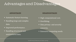
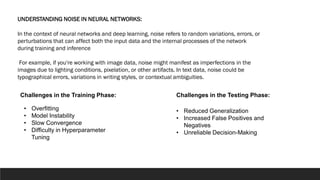
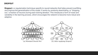
History of
Deep Learning
What is AI and ML?
Artificial Intelligence - a branch of
computer science by which we can create
intelligent machines which can behave like
a human, think like humans, and able to
make decisions.
Machine learning - enables a machine to
automatically learn from data, improve
performance from experiences, and predict
things without being explicitly
programmed.
CCS355 Neural Networks and Deep Learning
How Deep Learning is connected
with AI and ML?
▪ Deep Learning - a collection of statistical
techniques of machine learning for learning feature
hierarchies that are actually based on artificial
neural networks.
▪ It is the sub-branch of ML that helps to train ML
models with a huge amount of input and complex
algorithms and mainly works with neural
networks.
CCS355 Neural Networks and Deep Learning
DL ⊆ ML ⊆ AI
CCS355 Neural Networks and Deep Learning
How deep learning works?
Deep learning models consist of artificial neural networks with
multiple layers (hence the term "deep"). Each layer comprises
interconnected nodes (neurons) that transform input data into
progressively abstract representations.
The layers includes:
∘ Input Layer.
∘ Fully Connected (Dense) Layer.
∘ Convolutional Layer.
∘ Pooling (Subsampling) Layer.
∘ Recurrent Layer.
∘ Long Short-Term Memory (LSTM) Layer.
∘ Gated Recurrent Unit (GRU) Layer.
∘ Transformer Layer.
∘ Output Layer.
∘ Activation Function (e.g., ReLU, sigmoid, tanh).
∘ Batch Normalization Layer.
CCS355 Neural Networks and Deep Learning
Deep Learning History
• Deep learning has a rich and fascinating history. It emerged from the field of artificial intelligence and
neural networks. The concept of neural networks dates back to the 1940s and 1950s when
researchers attempted to mimic the human brain's structure in computational models.
• The term "deep learning" was coined in the 1980s by researchers such as Geoffrey Hinton.
However, progress was slow due to limited computational power and data availability. Neural
networks faced challenges in training and suffered from the vanishing gradient problem.
• In the mid-2000s, advancements in computational capabilities and the availability of large datasets
marked a turning point. Geoffrey Hinton and his team demonstrated the power of deep learning by
introducing the "deep belief network" and using it to win a pattern recognition competition in 2009.
• The real breakthrough came around 2012 when a deep learning algorithm called AlexNet won the
ImageNet competition, outperforming traditional computer vision approaches. This event triggered a
surge in interest and investment in deep learning.
• Since then, deep learning has become the dominant approach in various AI tasks, including computer
vision, natural language processing, and speech recognition. It has been instrumental in
revolutionizing fields like autonomous vehicles, healthcare, and many others.
• The development of deep learning has been driven by the collaborative efforts of researchers, the
availability of massive datasets, and advancements in hardware, particularly GPUs, which accelerated
the training process.
CCS355 Neural Networks and Deep Learning
Evolution of Deep Learning
CCS355 Neural Networks and Deep Learning
Types of Deep Learning Networks
∞ Convolutional Neural Networks (CNNs)
∞ Long Short Term Memory Networks (LSTMs)
∞ Recurrent Neural Networks (RNNs)
∞ Generative Adversarial Networks (GANs)
∞ Radial Basis Function Networks (RBFNs)
∞ Multilayer Perceptrons (MLPs)
∞ Self Organizing Maps (SOMs)
∞ Deep Belief Networks (DBNs)
∞ Restricted Boltzmann Machines( RBMs)
∞ Autoencoders
CCS355 Neural Networks and Deep Learning
Application
SELF DRIVING CARS
VOICE CONTROLLED
ASSISTANCE
COMPUTER VISION
NATURAL LANGUAGE
PROCESSING
FRAUD DETECTION
▪ The black-box problem.
▪ Lack of interpretability.
▪ Dependence on data quality.
▪ Lack of domain expertise.
▪ Unforeseen consequences.
Challenges
CCS355 Neural Networks and Deep Learning
Advantages and Disadvantages
ADVANTAGES
▪ Automatic feature learning.
▪ Handling large and complex
data.
▪ Improved performance.
▪ Handling structured and
unstructured data.
DISADVANTAGES
▪ High computational cost.
▪ Overfitting.
▪ Data privacy and security
concerns.
▪ Extensive computing needs.
CCS355 Neural Networks and Deep Learning
NOISE
ROBUSTNESS,
EARLY STOPPING,
BAGGING and
DROPOUT.
Regularization techniques provide us with a set of powerful tools to achieve this delicate balance.
In this seminar, we'll introduce you to some essential techniques that bolster the robustness and generalization
capabilities of our models.
We'll start by tackling the challenge of noise robustness, where we'll learn how to train models that remain
accurate even in the presence of noisy or uncertain data.
Then, we'll move on to the concept of early stoppingBagging comes next, an approach that leverages the
strength of multiple models to create a more accurate and resilient ensemble model. And finally, we'll delve into
dropout
INTRODUCTION:
In the context of neural networks and deep learning, noise refers to random variations, errors, or
perturbations that can affect both the input data and the internal processes of the network
during training and inference
For example, if you're working with image data, noise might manifest as imperfections in the
images due to lighting conditions, pixelation, or other artifacts. In text data, noise could be
typographical errors, variations in writing styles, or contextual ambiguities.
UNDERSTANDING NOISE IN NEURAL NETWORKS:
Challenges in the Training Phase:
• Overfitting
• Model Instability
• Slow Convergence
• Difficulty in Hyperparameter
Tuning
Challenges in the Testing Phase:
• Reduced Generalization
• Increased False Positives and
Negatives
• Unreliable Decision-Making
Techniques for Enhancing Noise Robustness:
1. Data Augmentation:
Data augmentation is a powerful technique to enhance noise robustness by artificially increasing the
diversity of the training dataset. It involves applying various transformations to the original data to create new
instances while preserving the underlying label or information. Here are some common data augmentation
methods:
Image Data: In image classification tasks, techniques like random cropping, rotation, flipping, brightness
adjustments, and adding noise can create variations of the same image. This helps the model learn to
recognize objects from different perspectives and lighting conditions.
Text Data: For natural language processing tasks, data augmentation involves techniques like synonym
replacement, sentence shuffling, and paraphrasing. These methods introduce variations in the text while
maintaining its semantic meaning.
Audio Data: In audio processing, techniques like time stretching, pitch shifting, and adding background noise
can create diverse audio samples for training speech recognition or sound classification models.
2. Regularization Techniques:
Regularization methods play a crucial role in enhancing noise robustness by preventing
overfitting and helping models generalize better in the presence of noise. Here's how some
regularization techniques contribute to noise robustness:
•L1 and L2 Regularization: These methods add penalty terms to the loss function based on
the magnitudes of the model's parameters. By encouraging smaller parameter values, they
reduce the model's sensitivity to noise and limit the impact of noisy features.
•Dropout: Dropout, which randomly deactivates neurons during training, introduces noise in
the learning process. This prevents the model from relying too heavily on specific neurons and
helps it learn more robust and adaptable features.
•Early Stopping: Early stopping prevents overfitting by monitoring the model's performance
on a validation set and stopping training when the performance starts to degrade. This
prevents the model from memorizing noise and encourages generalization.
•Batch Normalization: Batch normalization normalizes the inputs to a layer by adjusting the
mean and variance. This technique helps in stabilizing the training process and reducing the
impact of noise during learning.
To address these issues, regularization techniques come into play.
Techniques like dropout, weight decay, and early stopping help the model strike a balance
between fitting the training data and maintaining the ability to generalize.
By encouraging the model to focus on meaningful patterns and reducing its reliance on noise,
these techniques mitigate the risks of overfitting and enhance the model's generalization
capabilities.
Early stopping is a regularization technique used during the training of machine learning models,
particularly neural networks, to prevent overfitting and improve the model's generalization
performance. The idea behind early stopping is to monitor the model's performance on a separate
validation dataset during training and halt the training process once the model's performance on
the validation data starts deteriorating.
EARLY STOPPING:
Here's how early stopping works and why it's important:
Training Monitoring: During the training process, the model's performance metrics (such as
validation loss or accuracy) are tracked on a validation dataset that the model has not seen during
its training. This dataset serves as a proxy for how well the model will perform on new, unseen
data.
Early Stopping Criterion: Early stopping involves defining a stopping criterion based on the
validation performance. The training process continues until the validation performance starts to
degrade. This degradation is typically indicated by an increase in validation loss or a decrease in
validation accuracy.
Preventing Overfitting: When a model continues training for an extended period, it may start
fitting the noise or minor fluctuations in the training data. This results in improved performance on
the training data but worsened performance on unseen data. Early stopping prevents this
overfitting by stopping the training process when the model begins to over-optimize for the training
data at the expense of generalization.
Importance of Early Stopping:
Early stopping is crucial for several reasons:
1.Generalization: By stopping training at the optimal point, early stopping helps prevent
overfitting and ensures that the model can generalize well to new, unseen data.
2.Efficiency: Early stopping saves computational resources and time. Training deep learning
models can be time-consuming, and stopping once optimal generalization is achieved avoids
unnecessary training epochs.
3.Automatic Determination: Early stopping provides a principled way to determine the
appropriate number of training epochs without the need for manual trial and error.
4.Stability: It enhances the stability of the training process by avoiding unnecessary
fluctuations in model performance that can occur with continued training.
5.Flexibility: Early stopping can be implemented in various machine learning frameworks,
making it a practical and accessible technique for a wide range of practitioners.
The Role of Bagging in Reducing Variance
Bagging employs a simple yet ingenious concept: instead of relying on a single model, we create an ensemble
of models. Each model in the ensemble is trained on a different subset of the training data. This process
introduces diversity in the models' learning experiences and allows them to capture different facets of the
data's complexity.
Here's how it works:
Bootstrap Sampling: Bagging starts by randomly selecting multiple subsets of the training data with
replacement. This means that some data points might appear in multiple subsets, while others might not
appear at all. This creates diverse training sets for each model.
Model Training: Each subset is used to train a separate model. These models can be of the same type or
different types, depending on the problem at hand.
Combining Predictions: When it's time to make predictions, bagging combines the predictions of all individual
models in a way that reduces their individual errors and biases. This is typically done by averaging the
predictions for regression tasks or using voting for classification tasks.
Dropout is a regularization technique specific to neural networks that helps prevent overfitting
and improve the generalization of the model. It works by randomly deactivating, or "dropping
out," a fraction of neurons during each training iteration. This introduces a form of noise and
variability in the learning process, which encourages the network to become more robust and
adaptive.
DROPOUT
Here's how dropout works:
1.During Training:
1. For each training iteration, dropout randomly deactivates a portion of neurons in both the input
and hidden layers of the neural network. The deactivation is temporary and only occurs during
that specific iteration.
2. The probability of a neuron being dropped out is determined by a parameter called the dropout
rate, usually ranging from 0.2 to 0.5.
2.Effect on Forward Pass:
1. When neurons are dropped out, they do not contribute to the current forward pass of the data
through the network. This creates a "thinned" network for that iteration.
2. As a result, the remaining neurons must compensate for the missing ones, promoting the
learning of redundant features and preventing the network from relying too heavily on specific
neurons.
3.Effect on Backward Pass:
1. During the backward pass (backpropagation), only the active neurons participate in updating
the model's weights.
2. Dropout effectively makes the network behave as if it's an ensemble of several smaller
subnetworks. This ensemble-like behavior helps to combat overfitting
During Inference:
•During inference (when making predictions), dropout is not applied. Instead, the full network is used
to make predictions. However, the predictions are usually scaled by the inverse of the dropout rate to
account for the fact that more neurons are active during inference than during training.
Advantages of Regularization:
Overfitting Prevention: Regularization techniques effectively prevent overfitting, ensuring that models
generalize well to new, unseen data by avoiding the memorization of noise or irrelevant patterns.
Improved Generalization: Regularization enhances the model's ability to generalize by promoting the
learning of more relevant and robust features from the training data.
Stability: Regularization methods stabilize the training process by reducing the sensitivity of the model to
small changes in the training data, resulting in smoother convergence.
Simplicity: Many regularization techniques are easy to implement and integrate into existing machine
learning frameworks, requiring minimal additional effort.
Automatic Bias-Variance Trade-Off: Regularization techniques help strike a balance between bias and
variance, enabling models to find the optimal point that minimizes both underfitting and overfitting.
Disadvantages of Regularization:
Increased Complexity: Some regularization methods can introduce additional complexity to the model
architecture or training process, potentially increasing computational resources and time.
Hyperparameter Tuning: Properly tuning regularization hyperparameters (e.g., lambda in L2 regularization) can
require experimentation and understanding of the problem domain.
Model Interpretability: Certain regularization techniques, such as dropout or ensemble methods, might make
models less interpretable and harder to explain.
Resource Intensive: Techniques like ensembling or bagging involve training multiple models, which can be
resource-intensive in terms of memory and computation.
Limited Effect on Biased Data: Regularization might not fully address issues related to biased or unbalanced
datasets, where the inherent data distribution affects the model's performance.
Theoretical Understanding: Some regularization methods lack a clear theoretical understanding of why they
work, making it challenging to predict their effectiveness in all scenarios.
Enhancing noise robustness and optimizing techniques in neural networks and deep
learning is crucial for achieving reliable and accurate models. By understanding the
impact of noise, leveraging regularization, data augmentation, and optimizing network
training, we can mitigate noise interference and improve performance. Let's embrace
these techniques to unlock the full potential of neural networks in the presence of
noise.
CONCLUSION:
Chain Rule
And
BackPropagation
CCS355 Neural Networks and Deep Learning
Introduction To NN
Artificial Neural Networks (ANNs) are computational models
inspired by the human brain's neural structure. They consist of
interconnected nodes organized into layers, comprising an
input layer, one or more hidden layers, and an output layer.
The neurons within each layer process data and transfer it to
the subsequent layer.
The ultimate goal of neural networks is to learn from data and
make accurate predictions. This learning process involves
optimization techniques such as the Chain Rule and
Backpropagation.
CCS355 Neural Networks and Deep Learning
THE CHAIN RULE
• The Chain Rule is a fundamental calculus concept that facilitates the computation of derivatives for
composite functions.
• In the context of neural networks, it plays a crucial role in calculating the gradients of the network's
parameters during the training process.
• Given a composite function f(g(x)), the Chain Rule states that the derivative of the composite function can
be expressed as the product of the derivatives of its constituent functions:
(d/dx) f(g(x)) = f'(g(x)) * g'(x)
• This rule allows us to efficiently compute gradients through the layers of a neural network during the
Backpropagation process.
CCS355 Neural Networks and Deep Learning
1.Input Data: The forward pass begins with the input data, which could be a single sample or a batch of
samples. Each sample is represented as a feature vector.
2.Weighted Sum: For each neuron in a layer, the input data is multiplied by the corresponding weights of
the connections from the previous layer. These weighted sums are then summed up for each neuron.
3.Bias Addition: After the weighted sums are computed, a bias term is added to each neuron's sum. The
bias term provides a degree of freedom, allowing the model to shift the decision boundary.
4.Activation Function: Once the weighted sum and bias are calculated for each neuron, an activation
function is applied element-wise to the sums. The activation function introduces non-linearity to the
model, allowing it to learn complex patterns.
5.Output: The output of the activation function becomes the output of the current layer and is used as the
input for the next layer. The process repeats until the data has passed through all the layers in the network.
The output of the final layer is the predicted output of the neural network.
FORWARD PASS
CCS355 Neural Networks and Deep Learning
• Backpropagation is a learning algorithm used to train neural networks.
• Its objective is to minimize the error or loss function by adjusting the network's weights and biases.
• The process involves two main steps:
1.Forward Pass: The input data is propagated through the network to compute the predicted output.
2.Backward Pass: Gradients of the loss function with respect to the network's parameters (weights and
biases) are calculated using the Chain Rule.
Backpropagation: The Learning Algorithm
CCS355 Neural Networks and Deep Learning
Backpropagation Step-by-Step
1.Forward Pass
2. Calculate the Loss Function
3. Backward Pass
4. Compute Gradients for Weights and Biases
5.Update Weights and Biases
6. Iterative Process
CCS355 Neural Networks and Deep Learning
•Input data is fed into the neural network, and computations progress layer by layer from the input layer
to the output layer.
•Each neuron in a layer receives the weighted sum of inputs from the previous layer, including biases.
•The weighted sum is then passed through an activation function, introducing non-linearity and
generating the output of each neuron.
•This process is repeated for each layer until the final output is obtained.
1.Forward Pass
CCS355 Neural Networks and Deep Learning
•Once the forward pass is completed, the neural network produces its predicted output based on the
current weights and biases.
•The loss function, also known as the objective function or cost function, is applied to quantify the
difference between the predicted output and the ground truth (actual target).
•The loss function provides a measure of how well the model is performing on the training data.
2. Calculate the Loss Function
CCS355 Neural Networks and Deep Learning
•The backward pass is initiated to assess the impact of each network parameter (weights and biases) on
the overall loss.
•It involves analyzing the sensitivity of the loss function to changes in individual parameters, which
allows us to identify which parameters need adjustments to minimize the loss.
Chain Rule Application:
•At each layer during the backward pass, the Chain Rule comes into play.
•The Chain Rule is a mathematical principle that facilitates the computation of the derivative of a
composite function.
•In the context of Backpropagation, it enables us to calculate the partial derivatives of the loss function
concerning the weighted sum and the activation output of each neuron in the layer.
3. Backward Pass
CCS355 Neural Networks and Deep Learning
Gradients of Weights and Biases:
•Using the Chain Rule, the gradients of the loss with respect to each weight and bias in the layer are
computed.
•These gradients represent the sensitivity of the loss to changes in individual weights and biases.
•Larger gradient values indicate that a parameter has a more significant impact on the loss, and smaller
values suggest a lesser effect.
4. Compute Gradients for Weights and Biases
CCS355 Neural Networks and Deep Learning
•The gradients from each layer are accumulated and used to update the corresponding weights and biases.
•The optimization algorithm, such as Gradient Descent or its variants, leverages the accumulated
gradients to adjust the parameters.
•By moving the parameters in the direction of the negative gradient, the algorithm aims to minimize the
loss function.
5.Update Weights and Biases
CCS355 Neural Networks and Deep Learning
•The Backpropagation process is iterative, and it repeats for multiple epochs (iterations) during the
training phase.
•Each iteration involves a forward pass to compute predictions, a backward pass to calculate gradients,
and parameter updates using the optimization algorithm.
•Over multiple iterations, the neural network learns from the data, and the model's parameters are
gradually optimized for better predictions.
6. Iterative Process
CCS355 Neural Networks and Deep Learning
• Backpropagation can be implemented efficiently using matrix operations and vectorization.
• These techniques leverage parallelism and optimize the computation, making the training process
faster.
• The following steps are commonly used for Backpropagation implementation:
1.Matrix Multiplication: Represents the weighted inputs of neurons.
2.Vectorization: Enables parallelized calculations across multiple samples.
3.Element-wise Activation Functions: Applied to each neuron's output.
Implementation of Backpropagation
CCS355 Neural Networks and Deep Learning
• The Chain Rule and Backpropagation are indispensable components of training neural networks.
• They enable these models to learn complex patterns from data and have led to remarkable
advancements in artificial intelligence.
• Through the combined power of the Chain Rule and Backpropagation, neural networks have achieved
remarkable success in various real-world applications, such as image recognition, natural language
processing, and recommender systems.
Conclusion
CCS355 Neural Networks and Deep Learning
Batch Normalization
CCS355 Neural Networks and Deep Learning
What is batch normalization
• Batch Normalization – commonly abbreviated as Batch Norm – is one
of these methods.
• It is a widely used technique in the field of Deep Learning. It improves
the learning speed of Neural Networks and provides regularization,
avoiding overfitting.
CCS355 Neural Networks and Deep Learning
Normalization
• Normalization is a pre-processing technique used to
standardize data. In other words, having different sources of
data inside the same range.
• If we don’t normalizing the data before training can cause
problems in our network, making it drastically harder to train
and decrease its learning speed.
CCS355 Neural Networks and Deep Learning
Methods in normalization
METHOD 1:
• Method 1 to normalize our data ,The most straightforward
method is to scale it to a range from 0 to 1.
x →Data point to normalize.
m→ Mean
x max → Lowest value in dataset.
x max → Highest value in dataset.
CCS355 Neural Networks and Deep Learning
Method:2
The other technique Z-Score used to normalize data is forcing
the data points to have a mean of 0 and a standard deviation
of 1.
x →Data point to normalize.
m→ Mean
S → Standard deviation
Each data point mimics a standard normal distribution. Having
all the features on this scale, none of them will have a bias, and
therefore, our models will learn better.
CCS355 Neural Networks and Deep Learning
General format:
CCS355 Neural Networks and Deep Learning
Example
CCS355 Neural Networks and Deep Learning
Batch Normalization
• Batch Norm is a normalization technique done between the
layers of a Neural Network instead of in the raw data.
• It is done along mini-batches instead of the full data set. It
serves to speed up training and use higher learning rates,
making learning easier.
mz → mean of the neurons’ output
sz → standard deviation of the neurons’ output.
CCS355 Neural Networks and Deep Learning
How it works
In this image, we can see a regular feed-forward Neural Network
▪ X are the inputs
▪ z the output of the neurons
▪ a the output of the activation functions
▪ y the output of the network.
CCS355 Neural Networks and Deep Learning
Steps for Batch Normalization
• Batch Norm – in the image represented with a red line – is
applied to the neurons’ output just before applying the
activation function. Usually, a neuron without Batch Norm
would be computed as follows:
• Being g() he linear transformation of the neuron, w the weights
of the neuron, b the bias of the neurons, and f() activation
function. The model learns the parameters w and b Adding
Batch Norm, it looks as:
CCS355 Neural Networks and Deep Learning
Implementation in Python
• Implementing Batch Norm by using modern Machine Learning
frameworks such as Keras, Tensorflow.
CCS355 Neural Networks and Deep Learning
Why Does Batch Normalization
• Firstlynormalizing the inputs to take on a similar range of
values can speed up learning values in the layers of the
network, not only in the inputs.
• Batch Norm reduces the internal covariate shift (changes
during training and testing)of the network.
• example on the car rental service, imagine we want to include
other motorbikes.
CCS355 Neural Networks and Deep Learning
• If we only look at our previous data set, containing only cars,
our model will likely fail to predict motorbikes’ price. This
change in data (now containing motorbikes) is named
covariate shift, and it is gaining attention as it is a common
issue in real-world problems.
(Batch normalization will adapt to new features).
• Batch Norm has a regularization effect. Because it is
computed over mini-batches and not the entire data set, the
model’s data distribution sees each time has some noise. It
helps to overcome overfitting and help learn better.
CCS355 Neural Networks and Deep Learning
Advantages
• Stabilizing training.
• Higher learning rates
• Reduction of vanishing and
exploding gradients.
• Less sensitivity to weight
initialization.
• Regularization effect.
Disadvantages
• Batch size sensitivity- small size
leads to inaccurate value.
• Increased memory usage.
• Different calculation between
train and test.
CCS355 Neural Networks and Deep Learning
Gradient Learning
CCS355 NEURAL NETWORKS AND DEEP LEARNING
Gradient Learning
Gradient learning is a fundamental optimization
technique used in training neural networks. It
involves updating the parameters of the neural
network to minimize the difference between
the predicted output and the actual output, also
known as the loss or cost function
CCS355 NEURAL NETWORKS AND DEEP LEARNING
Cost Function
The cost function is defined as the measurement of difference or error between actual values
and expected values at the current position and present in the form of a single real number. It
helps to increase and improve machine learning efficiency by providing feedback to this model
so that it can minimize error and find the local or global minimum
The cost function is calculated after making a hypothesis with initial parameters and modifying
these parameters using gradient descent algorithms over known data to reduce the cost
function.
CCS355 NEURAL NETWORKS AND DEEP LEARNING
Backpropagation:
Backpropagation is a key technique used to compute the gradients efficiently in deep neural networks. It
is a two-phase process that involves the forward pass and the backward pass.
Forward Pass:
During the forward pass, the input data is fed into the neural network, and the activations of each layer
are computed using the current values of the parameters. The output of the network is compared with
the true labels, and the loss function is evaluated.
b. Backward Pass:
In the backward pass, the gradients of the loss function with respect to each parameter are calculated.
This is achieved using the chain rule of calculus to propagate the error from the output layer back to the
input layer. The gradients provide information about how the loss function changes with respect to
changes in the model's parameters.
CCS355 NEURAL NETWORKS AND DEEP LEARNING
Gradient Learning and Parameter Update:
Once the gradients are computed during backpropagation, gradient descent updates the model's
parameters to minimize the loss function. The general update equation for a parameter θ is:
θ_new = θ_old - learning_rate * gradient
where "learning_rate" is a hyperparameter that controls the step size of the updates. It
determines how much the parameters are adjusted in each iteration. A small learning rate can
lead to slow convergence, while a large learning rate can cause overshooting and divergence.
CCS355 NEURAL NETWORKS AND DEEP LEARNING
How does gradient descent works?
Before starting the working principle of gradient descent, we should know some basic concepts
to find out the slope of a line from linear regression. The equation for simple linear regression is
given as:
Y=mX+c
CCS355 NEURAL NETWORKS AND DEEP LEARNING
Learning Rate
It is defined as the step size taken to reach the minimum or lowest point. This is typically a small
value that is evaluated and updated based on the behavior of the cost function. If the learning
rate is high, it results in larger steps but also leads to risks of overshooting the minimum. At the
same time, a low learning rate shows the small step sizes, which compromises overall efficiency
but gives the advantage of more precision.
CCS355 NEURAL NETWORKS AND DEEP LEARNING
Types of Gradient Descent
Based on the error in various training models, the Gradient Descent
learning algorithm can be divided into
1. Batch gradient descent
2. stochastic gradient descent
3. mini-batch gradient descent.
CCS355 NEURAL NETWORKS AND DEEP LEARNING
1.Batch Gradient Descent
Batch gradient descent (BGD) is used to find the error for each point in the training set and update
the model after evaluating all training examples. This procedure is known as the training epoch. In
simple words, it is a greedy approach where we have to sum over all examples for each update.
Advantages of Gradient Descent
•It produces less noise in comparison to other gradient descent.
•It produces stable gradient descent convergence.
•It is Computationally efficient as all resources are used for all training samples.
CCS355 NEURAL NETWORKS AND DEEP LEARNING
2. Stochastic gradient descent
Stochastic gradient descent (SGD) is a type of gradient descent that runs one training example per iteration. Or in
other words, it processes a training epoch for each example within a dataset and updates each training example's
parameters one at a time. As it requires only one training example at a time, hence it is easier to store in allocated
memory. However, it shows some computational efficiency losses in comparison to batch gradient systems as it
shows frequent updates that require more detail and speed.
Advantages of Stochastic gradient descent
• It is easier to allocate in desired memory.
• It is relatively fast to compute than batch gradient descent
• It is more efficient for large datasets.
CCS355 NEURAL NETWORKS AND DEEP LEARNING
3. MiniBatch Gradient Descent
Mini Batch gradient descent is the combination of both batch gradient descent and stochastic gradient
descent. It divides the training datasets into small batch sizes then performs the updates on those batches
separately. Splitting training datasets into smaller batches make a balance to maintain the computational
efficiency of batch gradient descent and speed of stochastic gradient descent. Hence, we can achieve a special
type of gradient descent with higher computational efficiency and less noisy gradient descent.
Advantages of MiniBatch Gradient Descent
• It is easier to fit in allocated memory..
• It is computationally efficient.
• It produces stable gradient descent convergence.
CCS355 NEURAL NETWORKS AND DEEP LEARNING
CCS355 Neural Networks and Deep Learning
Recurrent Neural Network(RNN) is a type of Neural Network where the output from
the previous step is fed as input to the current step. In traditional neural networks, all the inputs and outputs are
independent of each other, but in cases when it is required to predict the next word of a sentence, the previous
words are required and hence there is a need to remember the previous words. Thus RNN came into existence,
which solved this issue with the help of a Hidden Layer. The main and most important feature of RNN is
its Hidden state, which remembers some information about a sequence. The state is also referred to as Memory
State since it remembers the previous input to the network. It uses the same parameters for each input as it
performs the same task on all the inputs or hidden layers to produce the output. This reduces the complexity of
parameters, unlike other neural networks.
CCS355 Neural Networks and Deep Learning
The Recurrent Neural Network consists of multiple fixed activation
function units, one for each time step. Each unit has an internal state which is
called the hidden state of the unit. This hidden state signifies the past knowledge
that the network currently holds at a given time step. This hidden state is updated
at every time step to signify the change in the knowledge of the network about the
past. The hidden state is updated using the following recurrence relation:-
where:
ht -> current state
ht-1 -> previous state
xt -> input state
CCS355 Neural Networks and Deep Learning
Yt -> output
Why -> weight at output layer
CCS355 Neural Networks and Deep Learning
L(θ)(loss function) depends on h3
h3 in turn depends on h2 and W
h2 in turn depends on h1 and W
h1 in turn depends on h0 and W
where h0 is a constant starting state.
CCS355 Neural Networks and Deep Learning

unit4 Neural Networks and Deep Learning.pdf

  • 1.
  • 2.
    What is AIand ML? Artificial Intelligence - a branch of computer science by which we can create intelligent machines which can behave like a human, think like humans, and able to make decisions. Machine learning - enables a machine to automatically learn from data, improve performance from experiences, and predict things without being explicitly programmed. CCS355 Neural Networks and Deep Learning
  • 3.
    How Deep Learningis connected with AI and ML? ▪ Deep Learning - a collection of statistical techniques of machine learning for learning feature hierarchies that are actually based on artificial neural networks. ▪ It is the sub-branch of ML that helps to train ML models with a huge amount of input and complex algorithms and mainly works with neural networks. CCS355 Neural Networks and Deep Learning
  • 4.
    DL ⊆ ML⊆ AI CCS355 Neural Networks and Deep Learning
  • 5.
    How deep learningworks? Deep learning models consist of artificial neural networks with multiple layers (hence the term "deep"). Each layer comprises interconnected nodes (neurons) that transform input data into progressively abstract representations. The layers includes: ∘ Input Layer. ∘ Fully Connected (Dense) Layer. ∘ Convolutional Layer. ∘ Pooling (Subsampling) Layer. ∘ Recurrent Layer. ∘ Long Short-Term Memory (LSTM) Layer. ∘ Gated Recurrent Unit (GRU) Layer. ∘ Transformer Layer. ∘ Output Layer. ∘ Activation Function (e.g., ReLU, sigmoid, tanh). ∘ Batch Normalization Layer. CCS355 Neural Networks and Deep Learning
  • 6.
    Deep Learning History •Deep learning has a rich and fascinating history. It emerged from the field of artificial intelligence and neural networks. The concept of neural networks dates back to the 1940s and 1950s when researchers attempted to mimic the human brain's structure in computational models. • The term "deep learning" was coined in the 1980s by researchers such as Geoffrey Hinton. However, progress was slow due to limited computational power and data availability. Neural networks faced challenges in training and suffered from the vanishing gradient problem. • In the mid-2000s, advancements in computational capabilities and the availability of large datasets marked a turning point. Geoffrey Hinton and his team demonstrated the power of deep learning by introducing the "deep belief network" and using it to win a pattern recognition competition in 2009. • The real breakthrough came around 2012 when a deep learning algorithm called AlexNet won the ImageNet competition, outperforming traditional computer vision approaches. This event triggered a surge in interest and investment in deep learning. • Since then, deep learning has become the dominant approach in various AI tasks, including computer vision, natural language processing, and speech recognition. It has been instrumental in revolutionizing fields like autonomous vehicles, healthcare, and many others. • The development of deep learning has been driven by the collaborative efforts of researchers, the availability of massive datasets, and advancements in hardware, particularly GPUs, which accelerated the training process. CCS355 Neural Networks and Deep Learning
  • 7.
    Evolution of DeepLearning CCS355 Neural Networks and Deep Learning
  • 8.
    Types of DeepLearning Networks ∞ Convolutional Neural Networks (CNNs) ∞ Long Short Term Memory Networks (LSTMs) ∞ Recurrent Neural Networks (RNNs) ∞ Generative Adversarial Networks (GANs) ∞ Radial Basis Function Networks (RBFNs) ∞ Multilayer Perceptrons (MLPs) ∞ Self Organizing Maps (SOMs) ∞ Deep Belief Networks (DBNs) ∞ Restricted Boltzmann Machines( RBMs) ∞ Autoencoders CCS355 Neural Networks and Deep Learning
  • 9.
    Application SELF DRIVING CARS VOICECONTROLLED ASSISTANCE COMPUTER VISION NATURAL LANGUAGE PROCESSING FRAUD DETECTION
  • 10.
    ▪ The black-boxproblem. ▪ Lack of interpretability. ▪ Dependence on data quality. ▪ Lack of domain expertise. ▪ Unforeseen consequences. Challenges CCS355 Neural Networks and Deep Learning
  • 11.
    Advantages and Disadvantages ADVANTAGES ▪Automatic feature learning. ▪ Handling large and complex data. ▪ Improved performance. ▪ Handling structured and unstructured data. DISADVANTAGES ▪ High computational cost. ▪ Overfitting. ▪ Data privacy and security concerns. ▪ Extensive computing needs. CCS355 Neural Networks and Deep Learning
  • 12.
  • 13.
    Regularization techniques provideus with a set of powerful tools to achieve this delicate balance. In this seminar, we'll introduce you to some essential techniques that bolster the robustness and generalization capabilities of our models. We'll start by tackling the challenge of noise robustness, where we'll learn how to train models that remain accurate even in the presence of noisy or uncertain data. Then, we'll move on to the concept of early stoppingBagging comes next, an approach that leverages the strength of multiple models to create a more accurate and resilient ensemble model. And finally, we'll delve into dropout INTRODUCTION:
  • 14.
    In the contextof neural networks and deep learning, noise refers to random variations, errors, or perturbations that can affect both the input data and the internal processes of the network during training and inference For example, if you're working with image data, noise might manifest as imperfections in the images due to lighting conditions, pixelation, or other artifacts. In text data, noise could be typographical errors, variations in writing styles, or contextual ambiguities. UNDERSTANDING NOISE IN NEURAL NETWORKS: Challenges in the Training Phase: • Overfitting • Model Instability • Slow Convergence • Difficulty in Hyperparameter Tuning Challenges in the Testing Phase: • Reduced Generalization • Increased False Positives and Negatives • Unreliable Decision-Making
  • 15.
    Techniques for EnhancingNoise Robustness: 1. Data Augmentation: Data augmentation is a powerful technique to enhance noise robustness by artificially increasing the diversity of the training dataset. It involves applying various transformations to the original data to create new instances while preserving the underlying label or information. Here are some common data augmentation methods: Image Data: In image classification tasks, techniques like random cropping, rotation, flipping, brightness adjustments, and adding noise can create variations of the same image. This helps the model learn to recognize objects from different perspectives and lighting conditions. Text Data: For natural language processing tasks, data augmentation involves techniques like synonym replacement, sentence shuffling, and paraphrasing. These methods introduce variations in the text while maintaining its semantic meaning. Audio Data: In audio processing, techniques like time stretching, pitch shifting, and adding background noise can create diverse audio samples for training speech recognition or sound classification models.
  • 16.
    2. Regularization Techniques: Regularizationmethods play a crucial role in enhancing noise robustness by preventing overfitting and helping models generalize better in the presence of noise. Here's how some regularization techniques contribute to noise robustness: •L1 and L2 Regularization: These methods add penalty terms to the loss function based on the magnitudes of the model's parameters. By encouraging smaller parameter values, they reduce the model's sensitivity to noise and limit the impact of noisy features. •Dropout: Dropout, which randomly deactivates neurons during training, introduces noise in the learning process. This prevents the model from relying too heavily on specific neurons and helps it learn more robust and adaptable features. •Early Stopping: Early stopping prevents overfitting by monitoring the model's performance on a validation set and stopping training when the performance starts to degrade. This prevents the model from memorizing noise and encourages generalization. •Batch Normalization: Batch normalization normalizes the inputs to a layer by adjusting the mean and variance. This technique helps in stabilizing the training process and reducing the impact of noise during learning.
  • 17.
    To address theseissues, regularization techniques come into play. Techniques like dropout, weight decay, and early stopping help the model strike a balance between fitting the training data and maintaining the ability to generalize. By encouraging the model to focus on meaningful patterns and reducing its reliance on noise, these techniques mitigate the risks of overfitting and enhance the model's generalization capabilities.
  • 18.
    Early stopping isa regularization technique used during the training of machine learning models, particularly neural networks, to prevent overfitting and improve the model's generalization performance. The idea behind early stopping is to monitor the model's performance on a separate validation dataset during training and halt the training process once the model's performance on the validation data starts deteriorating. EARLY STOPPING:
  • 19.
    Here's how earlystopping works and why it's important: Training Monitoring: During the training process, the model's performance metrics (such as validation loss or accuracy) are tracked on a validation dataset that the model has not seen during its training. This dataset serves as a proxy for how well the model will perform on new, unseen data. Early Stopping Criterion: Early stopping involves defining a stopping criterion based on the validation performance. The training process continues until the validation performance starts to degrade. This degradation is typically indicated by an increase in validation loss or a decrease in validation accuracy. Preventing Overfitting: When a model continues training for an extended period, it may start fitting the noise or minor fluctuations in the training data. This results in improved performance on the training data but worsened performance on unseen data. Early stopping prevents this overfitting by stopping the training process when the model begins to over-optimize for the training data at the expense of generalization.
  • 20.
    Importance of EarlyStopping: Early stopping is crucial for several reasons: 1.Generalization: By stopping training at the optimal point, early stopping helps prevent overfitting and ensures that the model can generalize well to new, unseen data. 2.Efficiency: Early stopping saves computational resources and time. Training deep learning models can be time-consuming, and stopping once optimal generalization is achieved avoids unnecessary training epochs. 3.Automatic Determination: Early stopping provides a principled way to determine the appropriate number of training epochs without the need for manual trial and error. 4.Stability: It enhances the stability of the training process by avoiding unnecessary fluctuations in model performance that can occur with continued training. 5.Flexibility: Early stopping can be implemented in various machine learning frameworks, making it a practical and accessible technique for a wide range of practitioners.
  • 21.
    The Role ofBagging in Reducing Variance Bagging employs a simple yet ingenious concept: instead of relying on a single model, we create an ensemble of models. Each model in the ensemble is trained on a different subset of the training data. This process introduces diversity in the models' learning experiences and allows them to capture different facets of the data's complexity. Here's how it works: Bootstrap Sampling: Bagging starts by randomly selecting multiple subsets of the training data with replacement. This means that some data points might appear in multiple subsets, while others might not appear at all. This creates diverse training sets for each model. Model Training: Each subset is used to train a separate model. These models can be of the same type or different types, depending on the problem at hand. Combining Predictions: When it's time to make predictions, bagging combines the predictions of all individual models in a way that reduces their individual errors and biases. This is typically done by averaging the predictions for regression tasks or using voting for classification tasks.
  • 22.
    Dropout is aregularization technique specific to neural networks that helps prevent overfitting and improve the generalization of the model. It works by randomly deactivating, or "dropping out," a fraction of neurons during each training iteration. This introduces a form of noise and variability in the learning process, which encourages the network to become more robust and adaptive. DROPOUT
  • 23.
    Here's how dropoutworks: 1.During Training: 1. For each training iteration, dropout randomly deactivates a portion of neurons in both the input and hidden layers of the neural network. The deactivation is temporary and only occurs during that specific iteration. 2. The probability of a neuron being dropped out is determined by a parameter called the dropout rate, usually ranging from 0.2 to 0.5. 2.Effect on Forward Pass: 1. When neurons are dropped out, they do not contribute to the current forward pass of the data through the network. This creates a "thinned" network for that iteration. 2. As a result, the remaining neurons must compensate for the missing ones, promoting the learning of redundant features and preventing the network from relying too heavily on specific neurons. 3.Effect on Backward Pass: 1. During the backward pass (backpropagation), only the active neurons participate in updating the model's weights. 2. Dropout effectively makes the network behave as if it's an ensemble of several smaller subnetworks. This ensemble-like behavior helps to combat overfitting During Inference: •During inference (when making predictions), dropout is not applied. Instead, the full network is used to make predictions. However, the predictions are usually scaled by the inverse of the dropout rate to account for the fact that more neurons are active during inference than during training.
  • 24.
    Advantages of Regularization: OverfittingPrevention: Regularization techniques effectively prevent overfitting, ensuring that models generalize well to new, unseen data by avoiding the memorization of noise or irrelevant patterns. Improved Generalization: Regularization enhances the model's ability to generalize by promoting the learning of more relevant and robust features from the training data. Stability: Regularization methods stabilize the training process by reducing the sensitivity of the model to small changes in the training data, resulting in smoother convergence. Simplicity: Many regularization techniques are easy to implement and integrate into existing machine learning frameworks, requiring minimal additional effort. Automatic Bias-Variance Trade-Off: Regularization techniques help strike a balance between bias and variance, enabling models to find the optimal point that minimizes both underfitting and overfitting.
  • 25.
    Disadvantages of Regularization: IncreasedComplexity: Some regularization methods can introduce additional complexity to the model architecture or training process, potentially increasing computational resources and time. Hyperparameter Tuning: Properly tuning regularization hyperparameters (e.g., lambda in L2 regularization) can require experimentation and understanding of the problem domain. Model Interpretability: Certain regularization techniques, such as dropout or ensemble methods, might make models less interpretable and harder to explain. Resource Intensive: Techniques like ensembling or bagging involve training multiple models, which can be resource-intensive in terms of memory and computation. Limited Effect on Biased Data: Regularization might not fully address issues related to biased or unbalanced datasets, where the inherent data distribution affects the model's performance. Theoretical Understanding: Some regularization methods lack a clear theoretical understanding of why they work, making it challenging to predict their effectiveness in all scenarios.
  • 26.
    Enhancing noise robustnessand optimizing techniques in neural networks and deep learning is crucial for achieving reliable and accurate models. By understanding the impact of noise, leveraging regularization, data augmentation, and optimizing network training, we can mitigate noise interference and improve performance. Let's embrace these techniques to unlock the full potential of neural networks in the presence of noise. CONCLUSION:
  • 27.
  • 28.
    Introduction To NN ArtificialNeural Networks (ANNs) are computational models inspired by the human brain's neural structure. They consist of interconnected nodes organized into layers, comprising an input layer, one or more hidden layers, and an output layer. The neurons within each layer process data and transfer it to the subsequent layer. The ultimate goal of neural networks is to learn from data and make accurate predictions. This learning process involves optimization techniques such as the Chain Rule and Backpropagation. CCS355 Neural Networks and Deep Learning
  • 29.
    THE CHAIN RULE •The Chain Rule is a fundamental calculus concept that facilitates the computation of derivatives for composite functions. • In the context of neural networks, it plays a crucial role in calculating the gradients of the network's parameters during the training process. • Given a composite function f(g(x)), the Chain Rule states that the derivative of the composite function can be expressed as the product of the derivatives of its constituent functions: (d/dx) f(g(x)) = f'(g(x)) * g'(x) • This rule allows us to efficiently compute gradients through the layers of a neural network during the Backpropagation process. CCS355 Neural Networks and Deep Learning
  • 30.
    1.Input Data: Theforward pass begins with the input data, which could be a single sample or a batch of samples. Each sample is represented as a feature vector. 2.Weighted Sum: For each neuron in a layer, the input data is multiplied by the corresponding weights of the connections from the previous layer. These weighted sums are then summed up for each neuron. 3.Bias Addition: After the weighted sums are computed, a bias term is added to each neuron's sum. The bias term provides a degree of freedom, allowing the model to shift the decision boundary. 4.Activation Function: Once the weighted sum and bias are calculated for each neuron, an activation function is applied element-wise to the sums. The activation function introduces non-linearity to the model, allowing it to learn complex patterns. 5.Output: The output of the activation function becomes the output of the current layer and is used as the input for the next layer. The process repeats until the data has passed through all the layers in the network. The output of the final layer is the predicted output of the neural network. FORWARD PASS CCS355 Neural Networks and Deep Learning
  • 31.
    • Backpropagation isa learning algorithm used to train neural networks. • Its objective is to minimize the error or loss function by adjusting the network's weights and biases. • The process involves two main steps: 1.Forward Pass: The input data is propagated through the network to compute the predicted output. 2.Backward Pass: Gradients of the loss function with respect to the network's parameters (weights and biases) are calculated using the Chain Rule. Backpropagation: The Learning Algorithm CCS355 Neural Networks and Deep Learning
  • 32.
    Backpropagation Step-by-Step 1.Forward Pass 2.Calculate the Loss Function 3. Backward Pass 4. Compute Gradients for Weights and Biases 5.Update Weights and Biases 6. Iterative Process CCS355 Neural Networks and Deep Learning
  • 33.
    •Input data isfed into the neural network, and computations progress layer by layer from the input layer to the output layer. •Each neuron in a layer receives the weighted sum of inputs from the previous layer, including biases. •The weighted sum is then passed through an activation function, introducing non-linearity and generating the output of each neuron. •This process is repeated for each layer until the final output is obtained. 1.Forward Pass CCS355 Neural Networks and Deep Learning
  • 34.
    •Once the forwardpass is completed, the neural network produces its predicted output based on the current weights and biases. •The loss function, also known as the objective function or cost function, is applied to quantify the difference between the predicted output and the ground truth (actual target). •The loss function provides a measure of how well the model is performing on the training data. 2. Calculate the Loss Function CCS355 Neural Networks and Deep Learning
  • 35.
    •The backward passis initiated to assess the impact of each network parameter (weights and biases) on the overall loss. •It involves analyzing the sensitivity of the loss function to changes in individual parameters, which allows us to identify which parameters need adjustments to minimize the loss. Chain Rule Application: •At each layer during the backward pass, the Chain Rule comes into play. •The Chain Rule is a mathematical principle that facilitates the computation of the derivative of a composite function. •In the context of Backpropagation, it enables us to calculate the partial derivatives of the loss function concerning the weighted sum and the activation output of each neuron in the layer. 3. Backward Pass CCS355 Neural Networks and Deep Learning
  • 36.
    Gradients of Weightsand Biases: •Using the Chain Rule, the gradients of the loss with respect to each weight and bias in the layer are computed. •These gradients represent the sensitivity of the loss to changes in individual weights and biases. •Larger gradient values indicate that a parameter has a more significant impact on the loss, and smaller values suggest a lesser effect. 4. Compute Gradients for Weights and Biases CCS355 Neural Networks and Deep Learning
  • 37.
    •The gradients fromeach layer are accumulated and used to update the corresponding weights and biases. •The optimization algorithm, such as Gradient Descent or its variants, leverages the accumulated gradients to adjust the parameters. •By moving the parameters in the direction of the negative gradient, the algorithm aims to minimize the loss function. 5.Update Weights and Biases CCS355 Neural Networks and Deep Learning
  • 38.
    •The Backpropagation processis iterative, and it repeats for multiple epochs (iterations) during the training phase. •Each iteration involves a forward pass to compute predictions, a backward pass to calculate gradients, and parameter updates using the optimization algorithm. •Over multiple iterations, the neural network learns from the data, and the model's parameters are gradually optimized for better predictions. 6. Iterative Process CCS355 Neural Networks and Deep Learning
  • 39.
    • Backpropagation canbe implemented efficiently using matrix operations and vectorization. • These techniques leverage parallelism and optimize the computation, making the training process faster. • The following steps are commonly used for Backpropagation implementation: 1.Matrix Multiplication: Represents the weighted inputs of neurons. 2.Vectorization: Enables parallelized calculations across multiple samples. 3.Element-wise Activation Functions: Applied to each neuron's output. Implementation of Backpropagation CCS355 Neural Networks and Deep Learning
  • 40.
    • The ChainRule and Backpropagation are indispensable components of training neural networks. • They enable these models to learn complex patterns from data and have led to remarkable advancements in artificial intelligence. • Through the combined power of the Chain Rule and Backpropagation, neural networks have achieved remarkable success in various real-world applications, such as image recognition, natural language processing, and recommender systems. Conclusion CCS355 Neural Networks and Deep Learning
  • 41.
    Batch Normalization CCS355 NeuralNetworks and Deep Learning
  • 42.
    What is batchnormalization • Batch Normalization – commonly abbreviated as Batch Norm – is one of these methods. • It is a widely used technique in the field of Deep Learning. It improves the learning speed of Neural Networks and provides regularization, avoiding overfitting. CCS355 Neural Networks and Deep Learning
  • 43.
    Normalization • Normalization isa pre-processing technique used to standardize data. In other words, having different sources of data inside the same range. • If we don’t normalizing the data before training can cause problems in our network, making it drastically harder to train and decrease its learning speed. CCS355 Neural Networks and Deep Learning
  • 44.
    Methods in normalization METHOD1: • Method 1 to normalize our data ,The most straightforward method is to scale it to a range from 0 to 1. x →Data point to normalize. m→ Mean x max → Lowest value in dataset. x max → Highest value in dataset. CCS355 Neural Networks and Deep Learning
  • 45.
    Method:2 The other techniqueZ-Score used to normalize data is forcing the data points to have a mean of 0 and a standard deviation of 1. x →Data point to normalize. m→ Mean S → Standard deviation Each data point mimics a standard normal distribution. Having all the features on this scale, none of them will have a bias, and therefore, our models will learn better. CCS355 Neural Networks and Deep Learning
  • 46.
    General format: CCS355 NeuralNetworks and Deep Learning
  • 47.
  • 48.
    Batch Normalization • BatchNorm is a normalization technique done between the layers of a Neural Network instead of in the raw data. • It is done along mini-batches instead of the full data set. It serves to speed up training and use higher learning rates, making learning easier. mz → mean of the neurons’ output sz → standard deviation of the neurons’ output. CCS355 Neural Networks and Deep Learning
  • 49.
    How it works Inthis image, we can see a regular feed-forward Neural Network ▪ X are the inputs ▪ z the output of the neurons ▪ a the output of the activation functions ▪ y the output of the network. CCS355 Neural Networks and Deep Learning
  • 50.
    Steps for BatchNormalization • Batch Norm – in the image represented with a red line – is applied to the neurons’ output just before applying the activation function. Usually, a neuron without Batch Norm would be computed as follows: • Being g() he linear transformation of the neuron, w the weights of the neuron, b the bias of the neurons, and f() activation function. The model learns the parameters w and b Adding Batch Norm, it looks as: CCS355 Neural Networks and Deep Learning
  • 51.
    Implementation in Python •Implementing Batch Norm by using modern Machine Learning frameworks such as Keras, Tensorflow. CCS355 Neural Networks and Deep Learning
  • 52.
    Why Does BatchNormalization • Firstlynormalizing the inputs to take on a similar range of values can speed up learning values in the layers of the network, not only in the inputs. • Batch Norm reduces the internal covariate shift (changes during training and testing)of the network. • example on the car rental service, imagine we want to include other motorbikes. CCS355 Neural Networks and Deep Learning
  • 53.
    • If weonly look at our previous data set, containing only cars, our model will likely fail to predict motorbikes’ price. This change in data (now containing motorbikes) is named covariate shift, and it is gaining attention as it is a common issue in real-world problems. (Batch normalization will adapt to new features). • Batch Norm has a regularization effect. Because it is computed over mini-batches and not the entire data set, the model’s data distribution sees each time has some noise. It helps to overcome overfitting and help learn better. CCS355 Neural Networks and Deep Learning
  • 54.
    Advantages • Stabilizing training. •Higher learning rates • Reduction of vanishing and exploding gradients. • Less sensitivity to weight initialization. • Regularization effect. Disadvantages • Batch size sensitivity- small size leads to inaccurate value. • Increased memory usage. • Different calculation between train and test. CCS355 Neural Networks and Deep Learning
  • 55.
    Gradient Learning CCS355 NEURALNETWORKS AND DEEP LEARNING
  • 56.
    Gradient Learning Gradient learningis a fundamental optimization technique used in training neural networks. It involves updating the parameters of the neural network to minimize the difference between the predicted output and the actual output, also known as the loss or cost function CCS355 NEURAL NETWORKS AND DEEP LEARNING
  • 57.
    Cost Function The costfunction is defined as the measurement of difference or error between actual values and expected values at the current position and present in the form of a single real number. It helps to increase and improve machine learning efficiency by providing feedback to this model so that it can minimize error and find the local or global minimum The cost function is calculated after making a hypothesis with initial parameters and modifying these parameters using gradient descent algorithms over known data to reduce the cost function. CCS355 NEURAL NETWORKS AND DEEP LEARNING
  • 58.
    Backpropagation: Backpropagation is akey technique used to compute the gradients efficiently in deep neural networks. It is a two-phase process that involves the forward pass and the backward pass. Forward Pass: During the forward pass, the input data is fed into the neural network, and the activations of each layer are computed using the current values of the parameters. The output of the network is compared with the true labels, and the loss function is evaluated. b. Backward Pass: In the backward pass, the gradients of the loss function with respect to each parameter are calculated. This is achieved using the chain rule of calculus to propagate the error from the output layer back to the input layer. The gradients provide information about how the loss function changes with respect to changes in the model's parameters. CCS355 NEURAL NETWORKS AND DEEP LEARNING
  • 59.
    Gradient Learning andParameter Update: Once the gradients are computed during backpropagation, gradient descent updates the model's parameters to minimize the loss function. The general update equation for a parameter θ is: θ_new = θ_old - learning_rate * gradient where "learning_rate" is a hyperparameter that controls the step size of the updates. It determines how much the parameters are adjusted in each iteration. A small learning rate can lead to slow convergence, while a large learning rate can cause overshooting and divergence. CCS355 NEURAL NETWORKS AND DEEP LEARNING
  • 60.
    How does gradientdescent works? Before starting the working principle of gradient descent, we should know some basic concepts to find out the slope of a line from linear regression. The equation for simple linear regression is given as: Y=mX+c CCS355 NEURAL NETWORKS AND DEEP LEARNING
  • 61.
    Learning Rate It isdefined as the step size taken to reach the minimum or lowest point. This is typically a small value that is evaluated and updated based on the behavior of the cost function. If the learning rate is high, it results in larger steps but also leads to risks of overshooting the minimum. At the same time, a low learning rate shows the small step sizes, which compromises overall efficiency but gives the advantage of more precision. CCS355 NEURAL NETWORKS AND DEEP LEARNING
  • 62.
    Types of GradientDescent Based on the error in various training models, the Gradient Descent learning algorithm can be divided into 1. Batch gradient descent 2. stochastic gradient descent 3. mini-batch gradient descent. CCS355 NEURAL NETWORKS AND DEEP LEARNING
  • 63.
    1.Batch Gradient Descent Batchgradient descent (BGD) is used to find the error for each point in the training set and update the model after evaluating all training examples. This procedure is known as the training epoch. In simple words, it is a greedy approach where we have to sum over all examples for each update. Advantages of Gradient Descent •It produces less noise in comparison to other gradient descent. •It produces stable gradient descent convergence. •It is Computationally efficient as all resources are used for all training samples. CCS355 NEURAL NETWORKS AND DEEP LEARNING
  • 64.
    2. Stochastic gradientdescent Stochastic gradient descent (SGD) is a type of gradient descent that runs one training example per iteration. Or in other words, it processes a training epoch for each example within a dataset and updates each training example's parameters one at a time. As it requires only one training example at a time, hence it is easier to store in allocated memory. However, it shows some computational efficiency losses in comparison to batch gradient systems as it shows frequent updates that require more detail and speed. Advantages of Stochastic gradient descent • It is easier to allocate in desired memory. • It is relatively fast to compute than batch gradient descent • It is more efficient for large datasets. CCS355 NEURAL NETWORKS AND DEEP LEARNING
  • 65.
    3. MiniBatch GradientDescent Mini Batch gradient descent is the combination of both batch gradient descent and stochastic gradient descent. It divides the training datasets into small batch sizes then performs the updates on those batches separately. Splitting training datasets into smaller batches make a balance to maintain the computational efficiency of batch gradient descent and speed of stochastic gradient descent. Hence, we can achieve a special type of gradient descent with higher computational efficiency and less noisy gradient descent. Advantages of MiniBatch Gradient Descent • It is easier to fit in allocated memory.. • It is computationally efficient. • It produces stable gradient descent convergence. CCS355 NEURAL NETWORKS AND DEEP LEARNING
  • 66.
    CCS355 Neural Networksand Deep Learning
  • 67.
    Recurrent Neural Network(RNN)is a type of Neural Network where the output from the previous step is fed as input to the current step. In traditional neural networks, all the inputs and outputs are independent of each other, but in cases when it is required to predict the next word of a sentence, the previous words are required and hence there is a need to remember the previous words. Thus RNN came into existence, which solved this issue with the help of a Hidden Layer. The main and most important feature of RNN is its Hidden state, which remembers some information about a sequence. The state is also referred to as Memory State since it remembers the previous input to the network. It uses the same parameters for each input as it performs the same task on all the inputs or hidden layers to produce the output. This reduces the complexity of parameters, unlike other neural networks. CCS355 Neural Networks and Deep Learning
  • 68.
    CCS355 Neural Networksand Deep Learning
  • 69.
    CCS355 Neural Networksand Deep Learning
  • 70.
    The Recurrent NeuralNetwork consists of multiple fixed activation function units, one for each time step. Each unit has an internal state which is called the hidden state of the unit. This hidden state signifies the past knowledge that the network currently holds at a given time step. This hidden state is updated at every time step to signify the change in the knowledge of the network about the past. The hidden state is updated using the following recurrence relation:- where: ht -> current state ht-1 -> previous state xt -> input state CCS355 Neural Networks and Deep Learning
  • 71.
    Yt -> output Why-> weight at output layer CCS355 Neural Networks and Deep Learning
  • 72.
    L(θ)(loss function) dependson h3 h3 in turn depends on h2 and W h2 in turn depends on h1 and W h1 in turn depends on h0 and W where h0 is a constant starting state. CCS355 Neural Networks and Deep Learning
  • 73.
    CCS355 Neural Networksand Deep Learning
  • 74.
    CCS355 Neural Networksand Deep Learning
  • 75.
    CCS355 Neural Networksand Deep Learning
  • 76.
    CCS355 Neural Networksand Deep Learning
  • 77.
    CCS355 Neural Networksand Deep Learning
  • 78.
    CCS355 Neural Networksand Deep Learning
  • 79.
    CCS355 Neural Networksand Deep Learning
  • 80.
    CCS355 Neural Networksand Deep Learning
  • 81.
    CCS355 Neural Networksand Deep Learning