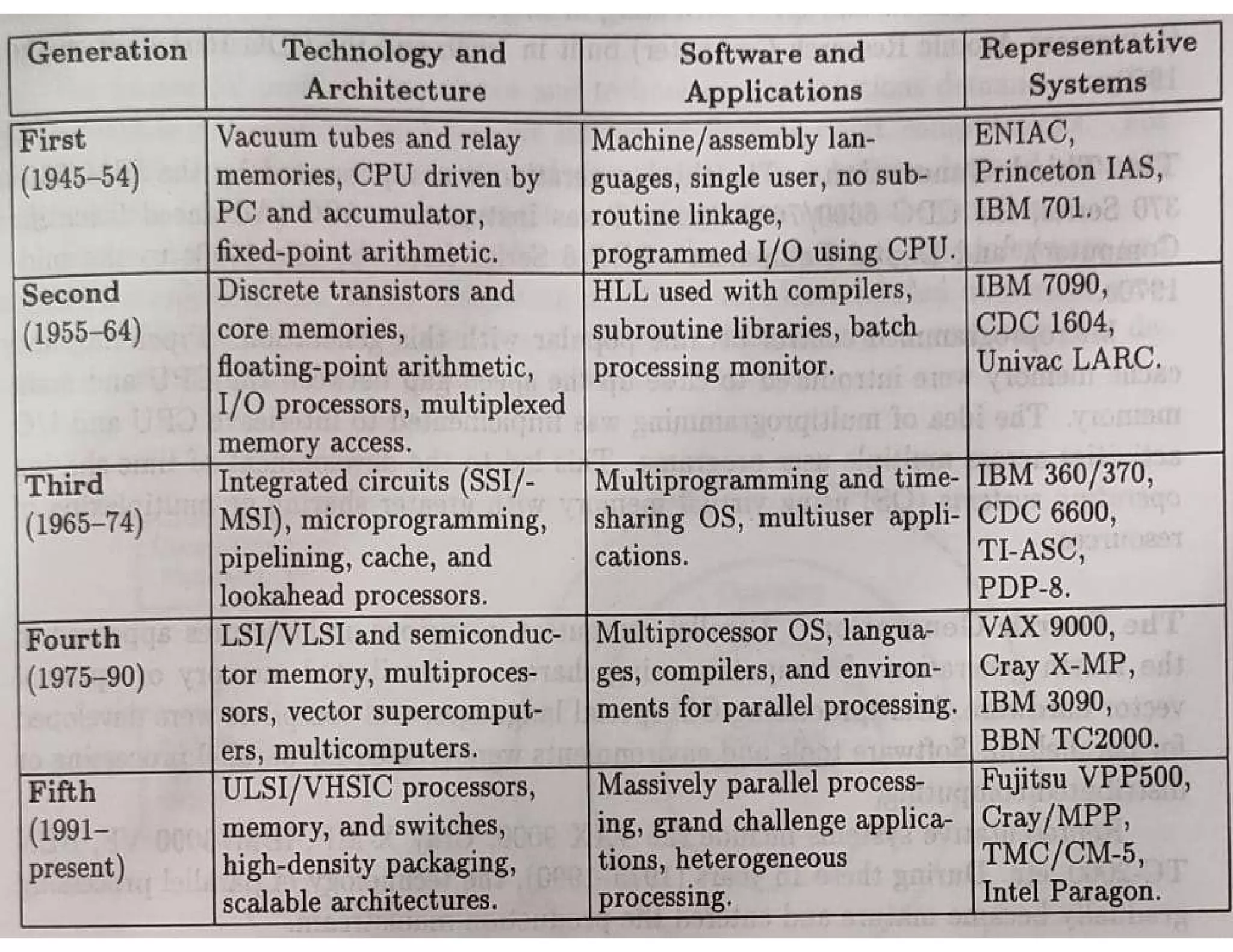
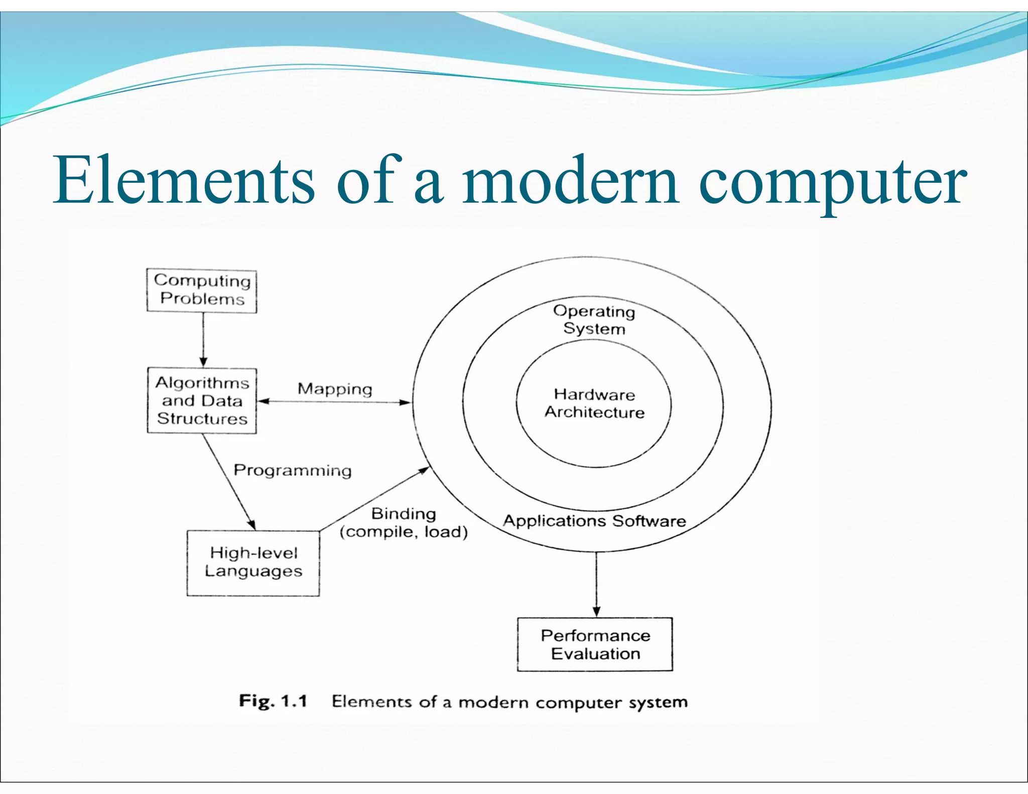
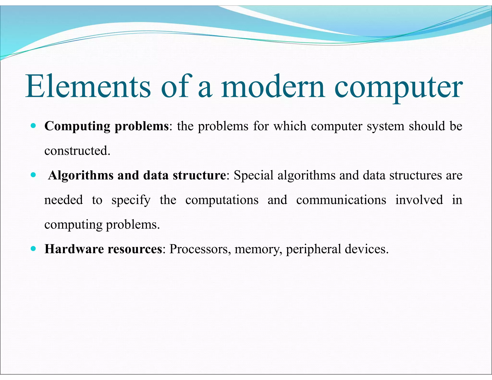
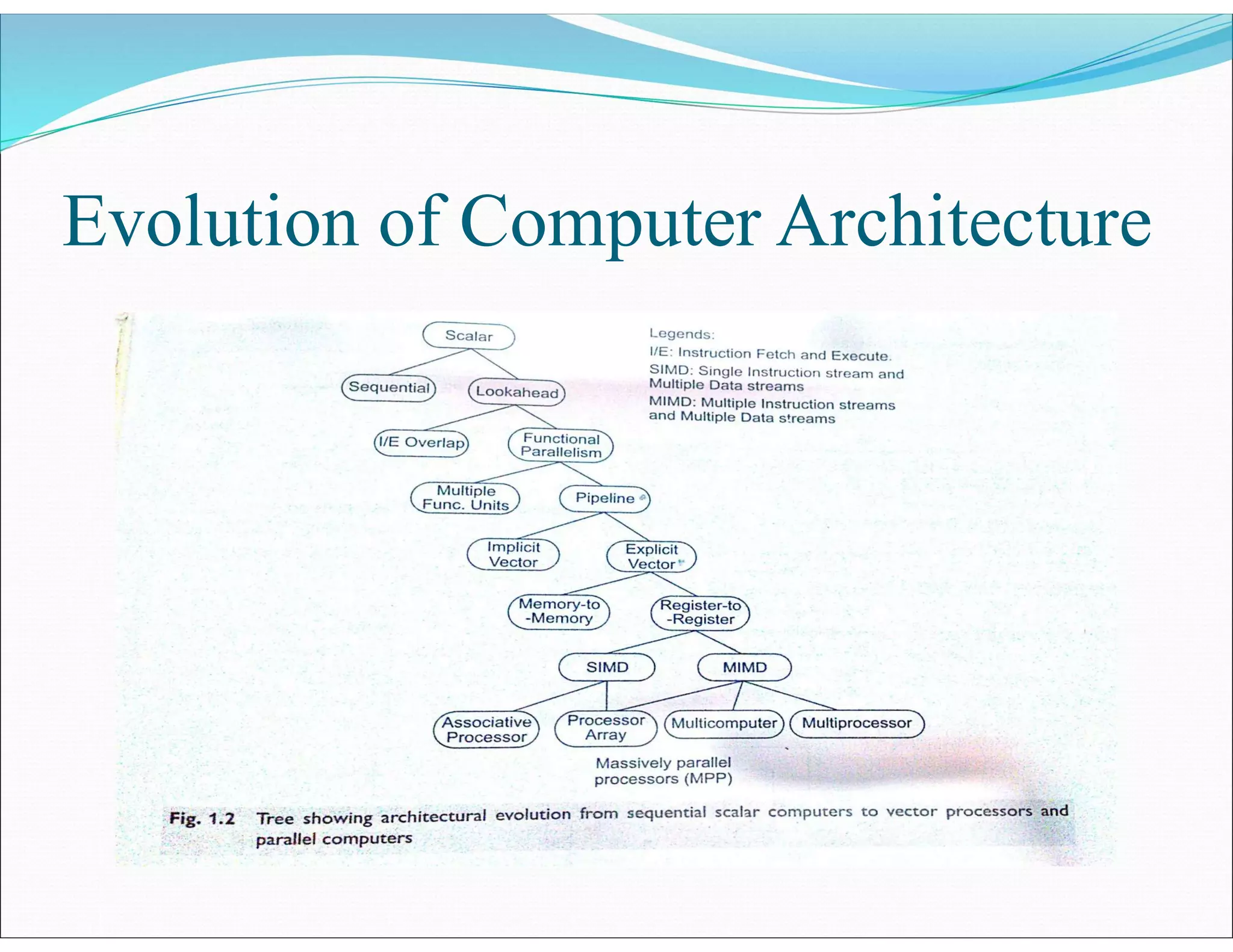
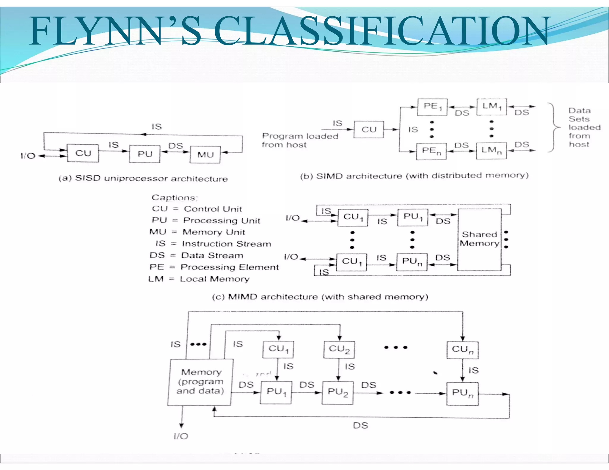
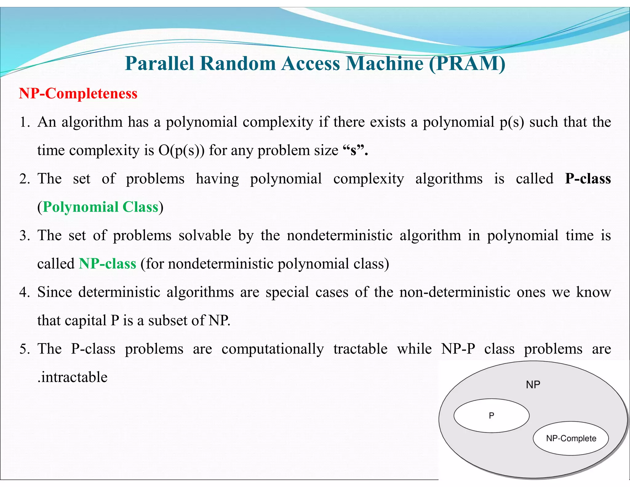
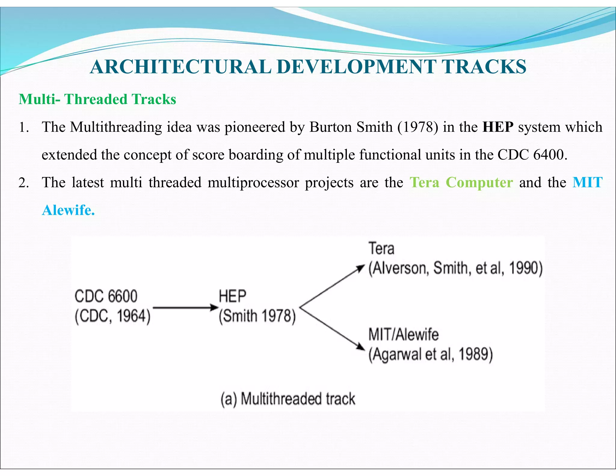
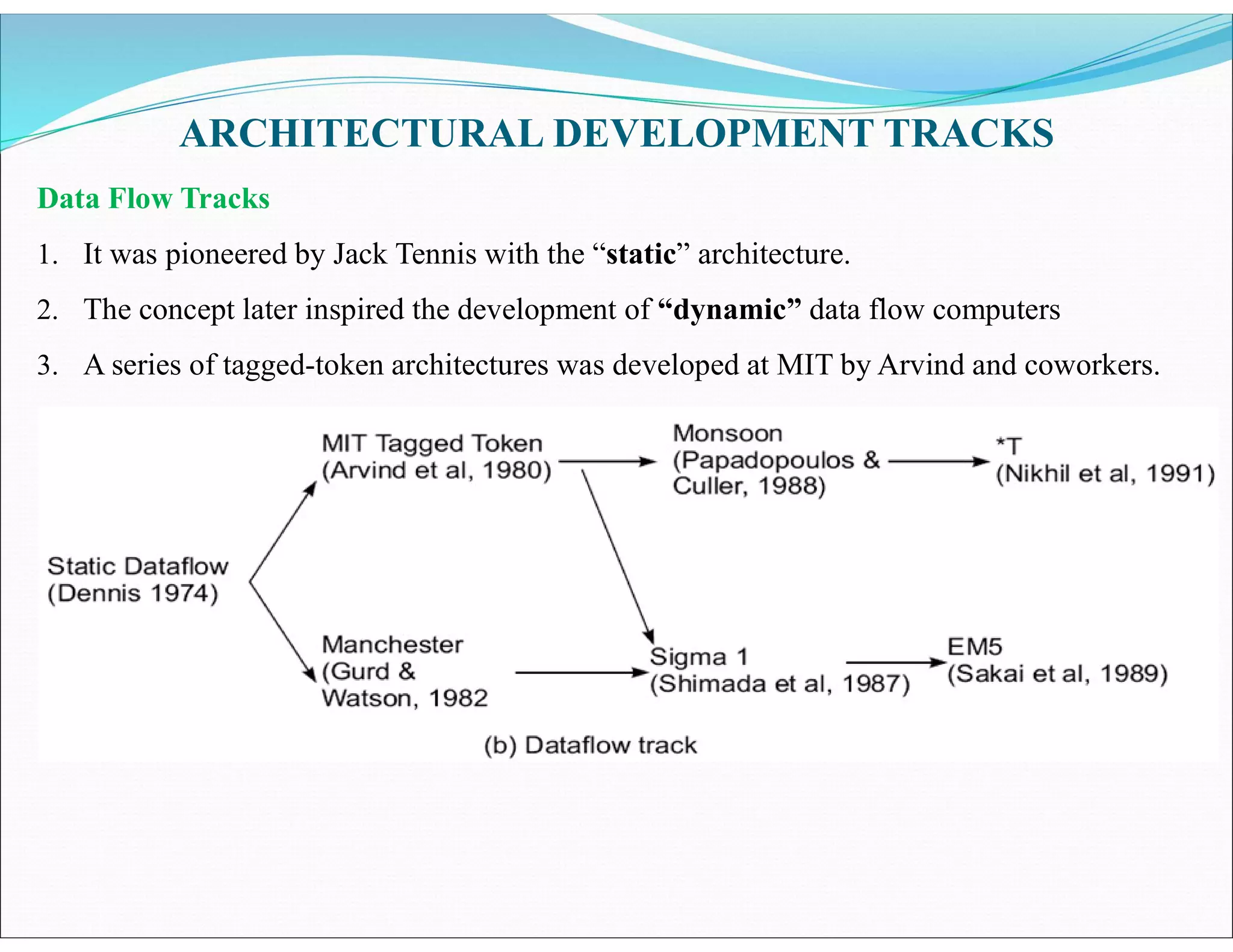
The document outlines essential elements of modern computer architecture, including computing problems, algorithms, hardware resources, and operating systems. It discusses the evolution of computer architecture, performance factors affecting system attributes, and classifications of parallel computing systems. Key concepts such as multi-processors, memory architecture models, PRAM models, and VLSI complexity are also reviewed.

4. Elements of a modern computer

5. Elements of a modern computer
 Computing problems: the problems for which computer system should be
constructed.
 Algorithms and data structure: Special algorithms and data structures are
needed to specify the computations and communications involved in
computing problems.
 Hardware resources: Processors, memory, peripheral devices.

6.  Operating system:
 System software support: Programs written in High level language. The
source code translated into object code by a compiler.
• Compiler support: 3 compiler approaches:
• 1. Prepocessor: uses a sequential compiler.
• 2. Precompiler: requires some program flow analysis, dependence checking
towards parallelism detection.
• 3. parallelizing compiler: demands a fully developed parallelizing compiler
which can automatically detect parallelism.

7. Evolution of Computer Architecture

8. FLYNN’S CLASSIFICATION

9. Parallel/Vector computers
 Execute programs on MIMD mode.
 2 major classes:
 1. shared-memory multiprocessors
 2. message-passing multicomputers.

10. System attributes to performance
 Turn around Time :-It is the time which includes disk
and memory access, input and output activities,
compilation time , OS overhead and CPU time.
 Clock rate and CPI: processor is driven by a clock
with a constant cycle time =t. The inverse of cycle
time is the clock rate (f=1/t).
 The size of the program is determined by its
instruction count. (Ic). Different machine instructions
may require different number of clock cycles to
execute. Therefore CPI (cycles per instruction)
becomes an important parameter.

11. Performance factors
 Ic= no. of instructions in a given program.
 Thus the CPU time needed to execute the program
is by finding the product of three factors:
T= Ic * CPI * t
 Instruction cycle requires cycle of events: instruction
fetch, decode, operand fetch, execution and store
results.

12.  In that cycle, only decode and execution phases are
carried out in the CPU. The remaining three
operations may require access to the memory.
 Therefore memory cycles is the time needed to
complete one memory reference.
 Therefore CPI is divided into 2 components=
processor cycles and memory cycles.
 Depending on the instruction type, the complete
instruction cycle may involve one to as many as four
memory references. (one for instruction fetch, two for
operand fetch, one for storing result).

13.  Therefore T= Ic * (p + m*k) * t
 Ic= instruction count
 P= number of processor cycles.
 M= number of memory references
 K= ratio between memory and processor cycle.
 t= processor cycle time
 T=CPU Time

14. System Attributes
 The 5 performance factors are influenced by 4
system attributes:
 Instruction-set architecture
 Compiler technology
 CPU implementation and control
 Cache and memory hierarchy

16.  Instruction-set architecture= Ic, p (processor cycle
per instruction)
 Compiler technology= Ic, p, m (memory references
per instruction)
 CPU implementation and control= p, t (processor
cycle time) total processor time needed.
 Cache and memory hierarchy= affects memory
access latency = k, t

17. MIPS RATE
 MIPS (millions instructions per second)
 Throughput rate: how many programs can a system
execute per unit time is called system throughput
Ws.
 In multiprogrammed, the system throughput is often
lower than the cpu throughput Wp.
 Because of additional system overheads caused by
the i/o, complier and os.

18. MIPS
 Let C be the total number of clock cycles needed to
execute a program.
 Therefore CPU time T= C*t= C/F
 Furthermore CPI= C/Ic
 T= CPI*Ic*t
 T= Ic*CPI/f
 The processor speed measured in MIPS.

19.  mips rate = Ic/T*10^6
 = f/CPI*10^6
 = f*Ic/ C*10^6
 F is clock rate/.
 Wp= f/Ic*CPI

20. Implicit and explicit parallelism

21.  Explicit parallelism requires more effort by the
programmer to develop a source program using
parallel dialects of C, C++, fortron, pascal.
Parallelism is specified in the user program. Here the
compiler needs to preserve the parallelism.

22. MULTI-PROCESSORS & MULTI COMPUTERS
1. Two categories of parallel computers
a. Shared memory multiprocessor
b. Distributed-memory multicomputer
Shared-memory multiprocessors:
1. The uniform memory access (UMA) model.
2. The non-uniform memory access (NUMA)
3. The cache-only memory architecture (COMA)
Note:
1. These models differ in how the memory and peripheral resources are shared or
distributed

23.  The physical memory is uniformly shared by all the processors. All
processors have equal access time to all memory words. Each processor
may use its own private cache.
 Peripherals are also shared in the same fashion.
 Multiprocessors are called tightly coupled systems due to high resource
sharing.
 The system interconnect takes the form of a shared bus, a crossbar switch,
or a multistage network. All the processors uniformly share the physical
memory
UNIFORM MEMORYACCESS

24. UNIFORM MEMORYACCESS

25. 1. UMA model is suitable for general-purpose and time-sharing applications.
2. When all processors have equal access time to all the peripheral devices,
the system is called a symmetric multiprocessor.
3. In an asymmetric multiprocessor, only one or a subset of processors are
executive capable.
4. An executive or master processor can execute the operating system and
handle I/O. The remaining processor has no I/O capabilities, and thus are
called the attached processors.

26. NUMA MODEL
 In this the access time varies with the location of the memory word. The shared
memory is physically distributed to all processors called local memories.
 The collection of all local memories forms a global address space accessible by all
processors.
 It is easier to access local memory with a local processor. The access of remote
memory attached to other processors takes longer due to added delay through the
interconnection network.
 There are 3 memory access patterns:
 Fastest is local memory access
 Next is global memory access
 Slowest is access to remote memory

28. COMA MODEL
 The COMA model is a particular case of a NUMA machine, in which the
distributed main memories are converted to caches.
 There is no memory hierarchy at each processor node.
 All the caches form a global address space. The distributed cache directories
assist remote cache access.
 Other variants of multiprocessor: CC-NUMA (Cache Coherent)

29. Distributed memory multi-computers
 The system consists of multiple computers often called nodes, Interconnected by
a message passing network.
 Each node is an autonomous computer consisting of:
 processor
 local memory and
 sometimes attached disc or I/O peripherals
 The message-passing network provides point-to-point static connections among
the nodes.
 All local memories are private and are accessible only by local processors.
 For this reason traditional multi-computers have been called no remote memory
access machines (NORMA)

30. Distributed memory multi-computers

31. MULTI COMPUTER GENERATIONS
 Message-passing multi-computers have gone through two generations of
development and a nee generation is developing.
 1st- 1983-1987- based on processor board technology using hypercube
architecture and s/w controlled message switching. E.g. Caltech Cosmic and
Intel iPSC/1.
 2nd 1988-1992- implemented with mesh-connected architecture and a software
environment for medium-grain distributed computing. E.g. Intel paragon and
the Parsys Supernode 1000.
 The 3rd 1992-1997 is expected to be a fine-grain multicomputer. E.g. MIT-J
Machine, Caltech Mosaic

32. VECOTR SUPER COMPUTERS
1. A vector computer is built on top of a scalar processor.
2. The vector processor is attached to the scalar processor as an optional feature
3. Program and data are first loaded into the main memory through a host computer.
4. All instructions are decoded by the
scalar control unit.
5. If scalar= goes to scalar processor.
6. If vector= sent to vector control unit.

33. VECTOR PROCESSOR MODEL
• The diagram shown is a register-to-register architecture.
• Vector registers are used to hold the vector operands, intermediate and final results.
• The vector functional pipelines retrieve operands from and put results into the
vector registers
• Each vector register is equipped with a component counter which keeps track of the
component registers used in successive pipeline cycles.
• The length of each vector register is usually fixed such as Cray series=fixed length
vector registers.
• Fujitsu VP2000= dynamically.
• Memory-to-memory= vector operands and results are directly retrieved and stored
from the main memory. E.g. 512 bits as in cyber 205.

34. SIMD SUPERCOMPUTERS
Operational Model
An operational model of a SIMD computer is specified by a tuple.
1. M = {N, C, I, M, R}
2. N = no. of processing elements (PEs).
3. C = set of instructions directly executed by the control unit (CU), including scalar and
program flow control instructions
4. I = is the set of instructions broadcast by the CU to all PEs for parallel execution. It
includes arithmetic, logic, data routing, masking, and other local operations executed
by each active PE over data within that PE
5. M = set of masking scheme, where mask partitions the set of PEs into enabled and
disabled.
6. R = set of data routing functions, specifying various patterns to be set up in the
interconnection network for Inter-PE communications.

36. PRAM AND VLSI MODELS
1. The ideal models provide a convenient framework for developing parallel algorithms
without worrying about the implementation details of physical constraints.
2. The models can be used to obtain the theoretical performance bounds on parallel
computers or to estimate VLSI complexity on-chip area and execution time before the
chip is fabricated.
Parallel Random Access Memory
1. Theoretical models of battle computers are:
a. Time and Space Complexities
b. NP-Completeness
c. PRAM Models

37. Parallel Random Access Machine (PRAM)
Time and Space complexity
1. The complexity of an algorithm for solving a problem of size “S” on a computer is determined
by the execution time and the storage space required.
Time Complexity
1. The time complexity is a function of the problem size.
2. The time complexity function in order notation is the asymptotic time complexity of the
algorithm.
3. Usually the worst-case time complexity is considered.
Space Complexity
1. The space complexity is defined as a function of the problem size “S”
2. The asymptotic space complexity refers to the data storage of large problems.
Note:
1. The program storage requirement and the storage for input data are not considered in this.
2. The time complexity of a serial algorithm is simply called serial complexity.
3. The time complexity of a parallel algorithm is called parallel complexity

38. Parallel Random Access Machine (PRAM)
NP-Completeness
1. An algorithm has a polynomial complexity if there exists a polynomial p(s) such that the
time complexity is O(p(s)) for any problem size “s”.
2. The set of problems having polynomial complexity algorithms is called P-class
(Polynomial Class)
3. The set of problems solvable by the nondeterministic algorithm in polynomial time is
called NP-class (for nondeterministic polynomial class)
4. Since deterministic algorithms are special cases of the non-deterministic ones we know
that capital P is a subset of NP.
5. The P-class problems are computationally tractable while NP-P class problems are
.intractable

39. PRAM Models
1. Conventional uni-processor computers were modeled as a random access machine
By Sheperdson and Sturgis (1963).
2. A Parallel random–access machine model (PRAM) has been developed by Fortune
and Wyllie for modeling idealized parallel computers with zero synchronization or
memory access overhead.
3. This PRAM model will be used for parallel algorithm development and for
scalability and complexity analysis.
4. An N- Processor PRAM has a globally addressable memory.
5. The shared memory can be distributed among the processors
or centralized In one place.
6. These processors work on synchronized read memory,
compute, and write memory cycles.

40. Which shared memory the model must specify how congruent read and congruent write of
memory is handled.
Four memory update options are possible
1. Exclusive read (ER)  This allows only one processor to read from any memory location
in each cycle.
2. Exclusive write (EW)  This allows at most one processor to write into a memory
location at a time.
3. Concurrent read (CR)  This allows multiple processors to read the same information
from the same memory cell in the same cycle.
4. Concurrent write (CW)  It allows simultaneous writes to the same memory. In order to
avoid confusion, some policies must be set up to resolve the right conflicts.
Note:
 Various combinations of the above options lead to several variants of the PRAM
model
PRAM Models

41. 1. EREW-PRAM model  This model forbids more than one processor from reading or
writing the same memory cell simultaneously.
2. CREW-PRAM model  The write conflicts are avoided by mutual exclusion. Current
reads to the same memory locations are allowed.
3. ERCW PRAM model  This allows exclusive read or concurrent write to the same
memory location
4. CRCW-PRAM model  This model allows either concurrent reads or concurrent writes
at the same time. The conflicting rights are resolved by one of the following four policies
a. Common  All simultaneous write stores the same value to the hot-spot memory location
b. Arbitrary  Any one of the values written may remain, the others are ignored.
c. Minimum  The value written by the processor with the minimum index will remain.
d. Priority  The value being written are combined using some associative functions such
as summation or maximum
PRAM VARIANTS

42. DISCREPANCY WITH PHYSICAL MODELS
1. PRAM models idealized parallel computers, in which all memory references and
program executions by multiple processors are synchronized without extra stock
cost. In reality, these models don’t exist
2. SIMD machine with shared memory is the closest architecture modeled by PRAM.
However, PRAM allows different instructions to be executed on different processors
simultaneously.
3. PRAM operates in synchronized MIMD mode with shared memory.
4. EREW and CRCW are the most popular models.
5. The CRCW algorithm runs faster than an equivalent EREW algorithm.
6. PRAM models will be used for scalability and performance comparison.
7. PRAM Models can put an upper bound and lower bound on the performance of a
system.

43. TO RESOLVE CONCURRENT WRITES
1. Common  all writes store the same value to the memory location.
2. Arbitrary  anyone of the values written may remain, the others are ignored.
3. Minimum  minimum value is selected.
4. Priority  the values written are combined using some associative functions such
as summation or maximum value.

44. VLSI COMPLEXITY MODEL


45. 

46. Memory Bound in a Chip Area A:
1. There are many computations that are memory bound, due to the need to process large
data sets.
2. The amount of information processed by the chip can be visualized as information flows
upward across the chip area.
3. Each bit can flow through a unit area of the horizontal chip slice. Thus the chip area
bounds the amount of memory bits stored on the chip.
I/O Bound on Volume AT:
1. The volume of the rectangular cube is represented by the product AT.
2. As information flows through the chip for a period of time T, the number of input bits
cannot exceed the volume.
3. This results in I/O limited lower bound on the product AT

47. 

48. ARCHITECTURAL DEVELOPMENT TRACKS
1. The architectures of most existing computers follow certain development tracks.
2. Understanding the features of various tracks provides insights for new architectural
developments. Some of them are:
Multi-Processor Tracks
A Multiprocessor system can be either a shared memory multi-processor or a distributed
memory multi-computer.
Shared Memory Track
1. The diagram represents a track of
multiprocessor development employing a single
address space in the entire system
2. The C.mmp was an UMA multiprocessor.
3. 16 PDP 11/40 processors are interconnected to
16 shared memory modules via crossbar switch

49. ARCHITECTURAL DEVELOPMENT TRACKS
Shared Memory Track
4. A special inter-processor interrupt is provided for fast inter-process communication besides
the shared memory, besides the shared memory.
5. The NYU Ultra-computer and Illinois Cedar projects were developed with a single address
space.
6. Both systems used multistage networks as
a system interconnect. The major
Achievements in the Cedar project are in
parallel compilers and performance
benchmarking experiments
7. The Standford Dash is a NUMA
multiprocessor with Distributed memories
forming a global address space

50. ARCHITECTURAL DEVELOPMENT TRACKS
Message Memory Track
1. The Cosmic Cube pioneered the development of message-passing computers
2. Since then Intel has provided a series of medium-grain hypercube computers
3. The nCUBE two also assumes a hypercube configuration.
4. The latest Intel system is the Paragon
5. On the research track the Mosaic C and the MIT J-Machine are the two fine grain multi
computers

51. ARCHITECTURAL DEVELOPMENT TRACKS
Multi-Vector and SIMD Tracks

52. ARCHITECTURAL DEVELOPMENT TRACKS
Multi-VectorTracks
1. These are traditional vectors in computers.
2. The CDC 7600 was the first vector dual processor system.
3. Two sub-tracks speed derived from the CDC 7600.
4. Cray 1 pioneered the multi-vector development in 1978
5. The latest cray/MPP is a massively parallel system with a distributed shared memory
6. It is supposed to work as a backend accelerator engine compatible with the existing Cray
Y-MP series

53. ARCHITECTURAL DEVELOPMENT TRACKS
SIMD Track
1. The Illiac IV pioneered the construction of SIMD computers, even the array processor
concept can be tracked far earlier to the 1960s.
2. The sub-track consisting of the Good Year MPP, the AMT/DAP610, and the TMC/CM-2,
are all SIMD machines built with the bit slice Pes.
3. The CM5 is a synchronized MIMD machine executing in a multiple SIMD mode.

54. ARCHITECTURAL DEVELOPMENT TRACKS
Multi- Threaded and Data Flow Tracks

55. ARCHITECTURAL DEVELOPMENT TRACKS
Multi- Threaded Tracks
1. The Multithreading idea was pioneered by Burton Smith (1978) in the HEP system which
extended the concept of score boarding of multiple functional units in the CDC 6400.
2. The latest multi threaded multiprocessor projects are the Tera Computer and the MIT
Alewife.

56. ARCHITECTURAL DEVELOPMENT TRACKS
Data Flow Tracks
1. It was pioneered by Jack Tennis with the “static” architecture.
2. The concept later inspired the development of “dynamic” data flow computers
3. A series of tagged-token architectures was developed at MIT by Arvind and coworkers.