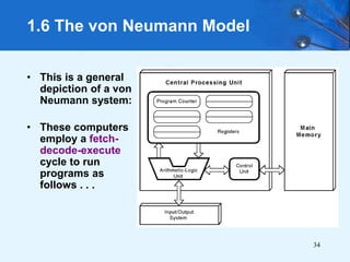
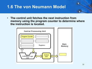
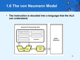
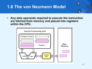
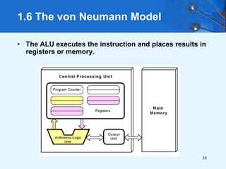
2. 2
Chapter 1 Objectives
Computer organization and architecture.
Units of measure common to computer systems.
Computer as a layered system.
Components von Neumann architecture and the
function of basic computer components.
3. 3
Why study computer organization and
architecture?
– understand and appreciate of a computer system’s
functional components, their characteristics, their
performance, and their interactions.
– to understand computer architecture in order to
make best use of the software tools and computer
languages they use to create programs.
– understand the complex trade-offs between CPU
clock speed, cache size, bus organization, number of
core processors, and so on
1.1 Overview
4. • Why study computer organization and
architecture?
– Computer architecture also underpins other
areas of the computing curriculum such as
operating systems (input/ output, memory
technology) and high-level languages (pointers,
parameter passing).
4
5. • The term architecture is taken to include
– instruction set architecture (the programmer’s
abstraction of a computer)
– organization or microarchitecture (the internal
implementation of a computer at the register
and functional unit level),
– system architecture (the organization of the
computer at the cache and bus level).
5
6. 6
1.1 Overview
• Computer organization
– physical aspects of computer systems.
– E.g., circuit design, control signals, memory types.
– How does a computer work?
• Computer architecture
– Logical aspects of system as seen by the programmer.
– E.g., instruction sets, instruction formats, data types,
addressing modes.
– How do I design a computer?
7. 7
1.2 Computer Components
• Principle of Equivalence of Hardware and
Software:
– Anything that can be done with software
can also be done with hardware, and
anything that can be done with hardware
can also be done with software.*
* Assuming speed is not a concern.
8. 8
• At the most basic level, a computer is a
device consisting of three pieces:
– A processor to interpret and execute programs
– A memory to store both data and programs
– A mechanism for transferring data to and from the
outside world.
1.2 Computer Components
10. 10
Measures of capacity and speed:
• Kilo- (K) = 1 thousand = 103 and 210
• Mega- (M) = 1 million = 106 and 220
• Giga- (G) = 1 billion = 109 and 230
• Tera- (T) = 1 trillion = 1012 and 240
• Peta- (P) = 1 quadrillion = 1015 and 250
1.3 An Example System
11. 11
• Hertz = clock cycles per second (frequency)
– 1MHz = 1,000,000Hz
– Processor speeds are measured in MHz or GHz.
• Byte = a unit of storage
– 1KB = 210 = 1024 Bytes
– 1MB = 220 = 1,048,576 Bytes
– Main memory (RAM) is measured in MB
– Disk storage is measured in GB for small systems, TB
for large systems.
1.3 An Example System
12. 12
1.3 An Example System
Measures of time and space:
• Milli- (m) = 1 thousandth = 10 -3
• Micro- () = 1 millionth = 10 -6
• Nano- (n) = 1 billionth = 10 -9
• Pico- (p) = 1 trillionth = 10 -12
• Femto- (f) = 1 quadrillionth = 10 -15
13. 13
• Millisecond = 1 thousandth of a second
– Hard disk drive access times are often 10 to 20
milliseconds.
• Nanosecond = 1 billionth of a second
– Main memory access times are often 50 to 70
nanoseconds.
• Micron (micrometer) = 1 millionth of a meter
– Circuits on computer chips are measured in microns.
1.3 An Example System
14. 14
Cycle time is the reciprocal of clock frequency.
A bus operating at 133MHz has a cycle time of 7.52
nanoseconds:
1.3 An Example System
Now back to the advertisement ...
133,000,000 cycles/second = 7.52ns/cycle
15. 15
1.3 An Example System
A system bus moves data within the
computer. The faster the bus the better.
This one runs at 400MHz.
The microprocessor is the “brain” of
the system. It executes program
instructions. This one is a Pentium
(Intel) running at 4.20GHz.
16. 16
1.3 An Example System
• Large main memory capacity means you can run
larger programs with greater speed than
computers having small memories.
• RAM = random access memory. Time to access
contents is independent of its location.
• Cache is a type of temporary memory that can
be accessed faster than RAM.
17. 17
1.3 An Example System
… and two levels of cache memory, the level 1 (L1)
cache is smaller and (probably) faster than the L2 cache.
Note that these cache sizes are measured in KB.
This system has 256MB of (fast)
synchronous dynamic RAM
(SDRAM) . . .
18. 18
1.3 An Example System
This one can store 80GB. 7200 RPM is the rotational
speed of the disk. Generally, the faster a disk rotates,
the faster it can deliver data to RAM. (There are many
other factors involved.)
Hard disk capacity determines
the amount of data and size of
programs you can store.
19. 19
1.3 An Example System
ATA stands for advanced technology attachment, which
describes how the hard disk interfaces with (or
connects to) other system components.
A CD can store about 650MB of data. This drive
supports rewritable CDs, CD-RW, that can be written
to many times.. 48x describes its speed.
20. 20
1.3 An Example System
This system has
ten ports.
Ports allow movement of data
between a system and its external
devices.
21. 21
1.3 An Example System
• Serial ports send data as a series of pulses along
one or two data lines.
• Parallel ports send data as a single pulse along
at least eight data lines.
• USB, Universal Serial Bus, is an intelligent serial
interface that is self-configuring. (It supports
“plug and play.”)
22. 22
1.3 An Example System
System buses can be augmented by
dedicated I/O buses. PCI, peripheral
component interface, is one such bus.
This system has three PCI devices: a video
card, a sound card, and a data/fax modem.
23. 23
1.3 An Example System
The number of times per second that the image on a
monitor is repainted is its refresh rate. The dot pitch
of a monitor tells us how clear the image is.
This one has a dot pitch of 0.24mm and a refresh rate of 75Hz.
The video card contains memory and
programs that support the monitor.
24. 24
• Writing complex programs requires a
“divide and conquer” approach, where
each program module solves a smaller
problem.
• Complex computer systems employ a
similar technique through a series of
virtual machine layers.
1.4 The Computer Level Hierarchy
25. 25
• Each virtual machine
layer is an abstraction of
the level below it.
• The machines at each
level execute their own
particular instructions,
calling upon machines at
lower levels to perform
tasks as required.
• Computer circuits
ultimately carry out the
work.
1.4 The Computer Level Hierarchy
26. 26
• Level 6: The User Level
– Program execution and user interface level.
– The level with which we are most familiar.
• Level 5: High-Level Language Level
– The level with which we interact when we write
programs in languages such as C, Pascal, Lisp, and
Java.
1.4 The Computer Level Hierarchy
27. 27
• Level 4: Assembly Language Level
– Acts upon assembly language produced from
Level 5, as well as instructions programmed
directly at this level.
• Level 3: System Software Level
– Controls executing processes on the system.
– Protects system resources.
– Assembly language instructions often pass
through Level 3 without modification.
1.4 The Computer Level Hierarchy
28. 28
• Level 2: Machine Level
– Also known as the Instruction Set Architecture
(ISA) Level.
– Consists of instructions that are particular to the
architecture of the machine.
– Programs written in machine language need no
compilers, interpreters, or assemblers.
1.4 The Computer Level Hierarchy
29. 29
• Level 1: Control Level
– A control unit decodes and executes instructions
and moves data through the system.
– Control units can be microprogrammed or
hardwired.
– A microprogram is a program written in a low-
level language that is implemented by the
hardware.
– Hardwired control units consist of hardware that
directly executes machine instructions.
1.4 The Computer Level Hierarchy
30. 30
• Level 0: Digital Logic Level
– This level is where we find digital circuits (the
chips).
– Digital circuits consist of gates and wires.
– These components implement the mathematical
logic of all other levels.
1.4 The Computer Level Hierarchy
31. 31
• On the Electronic Numerical Integrator and
Computer (ENIAC) that invented in 1946, all
programming was done at the digital logic level.
Programming the computer involved moving
plugs and wires.
• A different hardware configuration was needed
to solve every unique problem type.
1.6 The von Neumann Model
Configuring the ENIAC to solve a “simple” problem
required many days labor by skilled technicians.
32. 32
• The invention of stored program
computers has been ascribed to a
mathematician, John von Neumann,
who was a contemporary of Mauchley
and Eckert.
• Stored-program computers have
become known as von Neumann
Architecture systems.
1.6 The von Neumann Model
33. 33
1.6 The von Neumann Model
• Today’s stored-program computers have the
following characteristics:
– Three hardware systems:
• A central processing unit (CPU)
• A main memory system
• An I/O system
– The capacity to carry out sequential instruction
processing.
– A single data path between the CPU and main
memory.
• This single path is known as the von Neumann
bottleneck.
34. 34
1.6 The von Neumann Model
• This is a general
depiction of a von
Neumann system:
• These computers
employ a fetch-
decode-execute
cycle to run
programs as
follows . . .
35. 35
1.6 The von Neumann Model
• The control unit fetches the next instruction from
memory using the program counter to determine where
the instruction is located.
36. 36
1.6 The von Neumann Model
• The instruction is decoded into a language that the ALU
can understand.
37. 37
1.6 The von Neumann Model
• Any data operands required to execute the instruction
are fetched from memory and placed into registers
within the CPU.
38. 38
1.6 The von Neumann Model
• The ALU executes the instruction and places results in
registers or memory.
39. 39
• Conventional stored-program computers have
undergone many incremental improvements
over the years.
• These improvements include adding
specialized buses, floating-point units, and
cache memories, to name only a few.
• But enormous improvements in computational
power require departure from the classic von
Neumann architecture.
• Adding processors is one approach.
1.7 Non-von Neumann Models
40. 40
• In the late 1960s, high-performance computer
systems were equipped with dual processors
to increase computational throughput.
• In the 1970s supercomputer systems were
introduced with 32 processors.
• Supercomputers with 1,000 processors were
built in the 1980s.
• In 1999, IBM announced its Blue Gene
system containing over 1 million processors.
1.7 Non-von Neumann Models
41. 41
• Parallel processing is only one method
of providing increased computational
power.
• DNA computers, quantum computers,
and dataflow systems. At this point, it is
unclear whether any of these systems
will provide the basis for the next
generation of computers.
1.7 Non-von Neumann Models
42. 42
Leonard Adleman is often called the inventor of DNA
computers. His article in a 1994 issue of the journal Science
outlined how to use DNA to solve a well-known
mathematical problem, called the "traveling salesman"
problem. The goal of the problem is to find the shortest
route between a number of cities, going through each city
only once. As you add more cities to the problem, the
problem becomes more difficult. Adleman chose to find the
shortest route between seven cities. DNA computing is still
in its infancy.
1.7 Non-von Neumann Models
43. 43
• This chapter has given you an overview
of the subject of computer architecture.
Conclusion