Unit iii-Synchronization

Contents
Time and global states: Introduction – Clocks, events and process states –
Synchronizing physical clocks – Logical time and logical clocks – Global states –
Distributed debugging. Coordination and Agreement: Distributed mutual
exclusion – Elections – Multicast Communication.

Time and global states
Clocks, events and process states
● We take a distributed system to consist of a collection of N processes pi, i = 1, 2,...N.
● Each process executes on a single processor, and the processors do.not share memory
● Each process pi has a state si that, in general, it transforms as it executes. The process’s
state includes the values of all the variables within it.
● We define an event to be the occurrence of a single action that a process carries out as it
executes – a communication action or a state-transforming action.
● The sequence of events within a single process pi can be placed in a single, total ordering,
which we denote by the relation ->i between the events
● That is, e ->i e' if and only if the event e occurs before e’ at pi
● we can define the history of process pi to be the series of events that take place within it,
ordered as we have described by the relation ->i:

Clocks :
● Computers each contain their own physical clocks.
● These clocks are electronic devices that count oscillations occurring in a
crystal at a definite frequency, and typically divide this count and store
the result in a counter register.
● The operating system reads the node’s hardware clock value, Hi(t) ,
scales it and adds an offset so as to produce a software clock
● It approximately measures real, physical time t for process pi
● In other words, when the real time in an absolute frame of reference is
t, Ci(t) is the reading on the software clock
● In general, the clock is not completely accurate, so Ci)t􀀌 will differ from
t.

Clock skew and clock drift
Computer clocks, like any others, tend not to be in perfect agreement

Clock skew:
● The instantaneous difference between the readings of any two clocks is called their
skew.
● The difference between two clocks at any point in time is called clock skew

Clock drift:
● Clocks tick at different rate(count time at different rates)
● The phenomenon of clocks ticking at different rates. Creating a ever widening
gap is perceived time is known as clock drift
● Clock drift over the time is called “skew”

Coordinated Universal Time
● Computer clocks can be synchronized to external sources of highly accurate
time.
● The most accurate physical clocks use atomic oscillators, whose drift rate is
about one part in 10 pow 13.The output of these atomic clocks is used as the
standard for elapsed real time, known as International Atomic Time
● Coordinated Universal Time – abbreviated as UTC (from the French equivalent)
– is an international standard for timekeeping
● UTC signals are synchronized and broadcast regularly from landbased radio
stations and satellites covering many parts of the world.
● For example, in the USA, the radio station WWV(World Wide Vacuum)
broadcasts time signals on several shortwave frequencies. Satellite sources

Synchronizing physical clocks
We define these two modes of synchronization more closely as
follows, over an interval of real time I:
External synchronization means that all computers in the system
are synchronized with an external source of time (e.g., a UTC
signal).
Internal synchronization means that all computers in the system
are synchronized with one another, but the time is not necessarily
accurate with respect to UTC

•External synchronization
For a synchronization bound D>0, and for a source S of UTC time,
|S(t)-Ci(t)|<D for i-1,2,3,…N and for all real times t in I(where C is
computer’s clock)
•Internal synchronization
For a synchronization bound D>0 and Synchronized with other
computer in the distributed system |Ci(t)-Cj(t)|<D (where C is
computer’s clock) i,j=1,2,3…N and for all real times t in I

A clock that does not keep to whatever correctness conditions apply is defined to
be faulty. A clock’s crash failure is said to occur when the clock stops ticking
altogether; any other clock failure is an arbitrary failure. A historical example of
an arbitrary failure is that of a clock with the ‘Y2K bug’, which broke the
monotonicity condition by registering the date after 31 December 1999 as 1
January 1900 instead of 2000; another example is a clock whose batteries are
very low and whose drift rate suddenly becomes very large.

1.Synchronization in a synchronous system
● Internal synchronization between two processes in a synchronous
distributed system. In a synchronous system, bounds are known for the
drift rate of clocks, the maximum message transmission delay, and the
time required to execute each step of a process
● One process sends the time t on its local clock to the other in a message
m. In principle, the receiving process could set its clock to the time t
+ Ttrans , where Ttrans is the time taken to transmit m between them.
The two clocks would then agree (since the aim is internal
synchronization, it does not matter whether the sending process’s
clock is accurate).

● Unfortunately, Ttrans is subject to variation and is unknown. In
general, other processes are competing for resources with the
processes to be synchronized at their respective nodes, and other
messages compete with m for the network resources.
● Nonetheless, there is always a minimum transmission time, min, that
would be obtained if no other processes executed and no other
network traffic existed; min can be measured or conservatively
estimated.

● In a synchronous system, by definition, there is also an upper bound max
on the time taken to transmit any message.
● Let the uncertainty in the message transmission time be u, so that u =
(max – min). If the receiver sets its clock to be t + min , then the clock
skew may be as much as u, since the message may in fact have taken time
max to arrive. Similarly, if it sets its clock to t + max , the skew may
again be as large as u. If, however, it sets its clock to the halfway point,
t + (max + min)/2 , then the skew is at most u / 2 . In general, for a
synchronous system, the optimum bound that can be achieved on clock
skew when synchronizing N clocks is u(1 – 1 /N)

● Most distributed systems found in practice are asynchronous: the
factors leading to message delays are not bounded in their effect,
and there is no upper bound max on message transmission delays.
● This is particularly so for the Internet. For an asynchronous system,
we may say only that Ttrans = min + x , where x >= 0.

2.Cristian’s method for synchronizing clocks
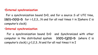
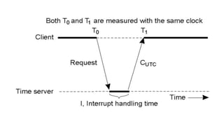
● Cristian [1989] suggested the use of a time server, connected to a device
that receives signals from a source of UTC, to synchronize computers
externally. Upon request, the server process S supplies the time
according to its clock, as shown in Figure 14.2

● A process p requests the time in a message mr , and receives the time
value t in a message mt
● Process p records the total round-trip time Tround taken to send the
request mr and receive the reply mt
● A simple estimate of the time to which p should set its clock is t +
Tround / 2 , which assumes that the elapsed time is split equally before
and after S placed t in mt .
● It is centralized passive time server type algorithm

● This algorithm suffers from the problem that afflicts all
single-server algorithms:
● the server might fail and clock synchronization will be
unavailable.

Berkeley algorithm
● Gusella and Zatti [1989] describe an algorithm for internal
synchronization that they developed for collections of computers running
Berkeley UNIX.
● In it, a coordinator computer is chosen to act as the master. Unlike in
Cristian’s protocol, this computer periodically polls the other computers
whose clocks are to be synchronized, called slaves. The slaves send back
their clock values to it.
● The master estimates their local clock times by observing the round-
trip times (similarly to Cristian’s technique), and it averages the values
obtained (including its own clock’s reading).

Instead of sending the updated current time back to the other computers – which
would introduce further uncertainty due to the message transmission time – the
master sends the amount by which each individual slave’s clock requires
adjustment. This can be a positive or negative value.
Average time=(2.50+3.25+3.00)/3=3.05

● Gusella and Zatti describe an experiment involving 15 computers whose
clocks were synchronized to within about 20–25 milliseconds using their
protocol. The local clocks’ drift rates were measured to be less than
2*10–5, and the maximum round-trip time was taken to be 10 milliseconds.
● Should the master fail, then another can be elected to take over and
function exactly as its predecessor.

The Network Time Protocol
● Cristian’s method and the Berkeley algorithm are intended primarily for use within intranets.
● The Network Time Protocol (NTP) [Mills 1995] defines an architecture for a time service and
a protocol to distribute time information over the Internet.
● NTP’s chief design aims and features are as follows:
○ To provide a service enabling clients across the Internet to be synchronized accurately
to UTC-NTP employs statistical techniques for the filtering of timing data and it
discriminates between the quality of timing data from different servers.
○ To provide a reliable service that can survive lengthy losses of connectivity-There are
redundant servers and redundant paths between the servers. The servers can
reconfigure so as to continue to provide the service if one of them becomes unreachable.
○ To enable clients to resynchronize sufficiently frequently to offset the rates of drift
found in most computers- The service is designed to scale to large numbers of clients
and servers.
○ To provide protection against interference with the time service, whether malicious or
accidental- The time service uses authentication techniques to check that timing data
originate from the claimed trusted sources. It also validates the return addresses of
messages sent to it.

● The NTP service is provided by a network of servers located across the
Internet.
● Primary servers are connected directly to a time source such as a radio
clock receiving UTC;
● Secondary servers are synchronized, ultimately, with primary servers.
The servers are connected in a logical hierarchy called a “synchronization
subnet” whose levels are called strata. Primary servers occupy stratum 1:
they are at the root.
● Stratum 2 servers are secondary servers that are synchronized directly
with the primary servers;
● stratum 3 servers are synchronized with stratum 2 servers, and so on.
The lowest-level (leaf) servers execute in users’ workstations.

● The clocks belonging to servers with high stratum numbers are liable to be
less accurate than those with low stratum numbers, because errors are
introduced at each level of synchronization.
● NTP also takes into account the total message round-trip delays to the
root in assessing the quality of timekeeping data held by a particular server.
● The synchronization subnet can reconfigure as servers become unreachable
or failures occur.
● If, for example, a primary server’s UTC source fails, then it can become a
stratum 2 secondary server. If a secondary server’s normal source of
synchronization fails or becomes unreachable, then it may synchronize with
another server.
● NTP servers synchronize with one another in one of three modes:
multicast, procedure-call and symmetric mode

Multicast mode is intended for use on a high-speed LAN. One or more
servers periodically multicasts the time to the servers running in other
computers connected by the LAN, which set their clocks assuming a small
delay. This mode can achieve only relatively low accuracies, but ones that
nonetheless are considered sufficient for many purposes.
Procedure-call mode is similar to the operation of Cristian’s algorithm, In
this mode, one server accepts requests from other computers, which it
processes by replying with its timestamp (current clock reading). This mode is
suitable where higher accuracies are required than can be achieved with
multicast, or where multicast is not supported in hardware. For example, file
servers on the same or a neighbouring LAN that need to keep accurate timing
information for file accesses could contact a local server in procedure-call
mode.

Finally, symmetric mode is intended for use by the servers that supply time
information in LANs and by the higher levels (lower strata) of the synchronization
subnet, where the highest accuracies are to be achieved. A pair of servers
operating in symmetric mode exchange messages bearing timing information.
Timing data are retained as part of an association between the servers that is
maintained in order to improve the accuracy of their synchronization over time.
In all modes, messages are delivered unreliably, using the standard UDP Internet
transport protocol. In procedure-call mode and symmetric mode, processes
exchange pairs of messages. Each message bears timestamps of recent message
events: the local times when the previous NTP message between the pair was sent
and received, and the local time when the current message was transmitted

● The recipient of the NTP message notes the local time when it receives
the message. The four times Ti – 3 , Ti – 2 , Ti – 1 and Ti are shown
in Figure 14.4
● Messages exchanged between a pair of NTP peers for the messages m
and m' sent between servers A and B.
● Note that in symmetric mode, unlike in Cristian’s algorithm, there can be
a nonnegligible delay between the arrival of one message and the dispatch
of the next. Also, messages may be lost, but the three timestamps
carried by each message are nonetheless valid.

● For each pair of messages sent between two servers the NTP calculates an offset oi ,
which is an estimate of the actual offset between the two clocks.
● If the true offset of the clock at B relative to that at A is o, and if the actual
transmission times for m and m' are t and t', respectively, then we have:
Ti – 2 = Ti – 3 + t + o and Ti = Ti – 1 + t’– o
t=Ti-2-Ti-3-o t’=Ti-Ti-1+o
● This leads to:(delay di , which is the total transmission time for the two messages. )
di = t + t’ = Ti – 2 – Ti – 3 + Ti – Ti – 1
● And:
o = oi + (t’ – t)/ 2 , where oi = (Ti – 2 – Ti – 3 + Ti – 1 – Ti)/2
● Using the fact that t, t’>= 0 , it can be shown that oi – di / 2 <=o <= oi + di / 2 . Thus oi is
an estimate of the offset, and di is a measure of the accuracy of this estimate.

● NTP servers apply a data filtering algorithm to successive pairs <oi, di>, which estimates the
offset o and calculates the quality of this estimate as a statistical quantity called the filter
dispersion.
● A relatively high filter dispersion represents relatively unreliable data. The eight most recent
pairs <oi, di> are retained. As with Cristian’s algorithm, the value of oj that corresponds to the
minimum value dj is chosen to estimate o.
● In general, an NTP server engages in message exchanges with several of its peers. In
addition to data filtering applied to exchanges with each single peer, NTP applies a peer-
selection algorithm. This examines the values obtained from exchanges with each of several
peers, looking for relatively unreliable values. The output from this algorithm may cause a
server to change the peer that it primarily uses for synchronization.
● Peers with lower stratum numbers are more favoured than those in higher strata because they
are ‘closer’ to the primary time sources.
● Also, those with the lowest synchronization dispersion are relatively favoured. This is the sum
of the filter dispersions measured between the server and the root of the synchronization
subnet.

● NTP employs a phase lock loop model [Mills 1995], which modifies the
local clock’s update frequency in accordance with observations of its
drift rate. To take a simple example, if a clock is discovered always to
gain time at the rate of, say, four seconds per hour, then its frequency
can be reduced slightly (in software or hardware) to compensate for this.
The clock’s drift in the intervals between synchronization is thus
reduced.
● Mills quotes synchronization accuracies on the order of tens of
milliseconds over Internet paths, and one millisecond on LANs

Logical time and logical clocks
● From the point of view of any single process, events are ordered uniquely
by times shown on the local clock. However, as Lamport [1978] pointed out,
since we cannot synchronize clocks perfectly across a distributed system, we
cannot in general use physical time to find out the order of any arbitrary pair
of events occurring within it.
● In general, we can use a scheme that is similar to physical causality but that
applies in distributed systems to order some of the events that occur at
different processes. This ordering is based on two simple and intuitively
obvious points:
○ If two events occurred at the same process pi (i = 1, 2, .. N), then they
occurred in the order in which pi observes them – this is the order ->i
that we defined above.
○ Whenever a message is sent between processes, the event of sending
the message occurred before the event of receiving the message

Lamport called the partial ordering obtained by generalizing these two
relationships the happened-before relation. It is also sometimes known as the
relation of causal ordering or potential causal ordering.

● The relation -> is illustrated for the case of three processes, p1 , p2 and p3. It
can be seen that a -> b, since the events occur in this order at process p1 (a ->i b), and
similarly c -> d. Furthermore, b -> c, since these events are the sending and reception
of message m1 , and similarly d -> f. Combining these relations, we may also say that,
for example, a -> f.
● It can also be seen from Figure 14.5 that not all events are related by the relation ->.
For example, a e and e a, since they occur at different processes, and there is no
chain of messages intervening between them. We say that events such as a and e that
are not ordered by -> are concurrent and write this a||e .
● The relation -> captures a flow of data intervening between two events

Logical clocks
● Lamport [1978] invented a simple mechanism by which the happened
before ordering can be captured numerically, called a logical clock.
● A Lamport logical clock is a monotonically increasing software counter,
whose value need bear no particular relationship to any physical clock.
● Each process pi keeps its own logical clock, Li , which it uses to apply so-
called Lamport timestamps to events.
● We denote the timestamp of event e at pi by Li(e) , and by L(e) we
denote the timestamp of event e at whatever process it occurred at.

● Although we increment clocks by 1, we could have chosen any positive value. It can
easily be shown, by induction on the length of any sequence of events relating two
events e and e’ , that e -> e’ L(e)<L(e’) .
● Note that the converse is not true. If L(e)< L(e’), then we cannot infer that e -
> e’ .Each of the processes p1 , p2 and p3 has its logical clock initialized to 0. The
clock values given are those immediately after the event to which they are
adjacent. Note that, for example, L(e)< L(b) but b || e .

Totally ordered logical clocks(unique Time stamp)
● In the figure, A timestamp of 1 is associated with events a and e in the
process p1 and p3 respectively
● The times may be same but the events are distinct
● Create a total order by attaching the process number to an event
● If e is an event occurring at pi with local timestamp Ti , and e’ is an event
occurring at pj with local timestamp Tj , we define the global logical
timestamps for these events to be (Ti, i) and (Tj, j) , respectively. And
we define (Ti, i) < (Tj, j) if and only if either Ti < Tj , or Ti = Tj and i <
j .

Vector clocks
● Mattern [1989] and Fidge [1991] developed vector clocks to overcome
the shortcoming of Lamport’s clocks: the fact that from L(e) < L(e’) we
cannot conclude that e -> e’·
● A vector clock for a system of N processes is an array of N integers.
● Each process keeps its own vector clock, Vi , which it uses to timestamp
local events.
● Like Lamport timestamps, processes piggyback vector timestamps on the
messages they send to one another, and there are simple rules for
updating the clocks

● Vector initialized to 0 at each process
● Process increments its element of the vector in local vector before
timestamping event:
Vi[i]=vi[i]+1
● Message is sent from process pi with vi attached to it
● When pj receives message compares vectors element by element and
sets local vector to higher of two values
Vj[i]=max(Vi[i],Vj[i]) for i=1,...N

Let V(e) be the vector timestamp applied by the process at which e occurs. It is
straightforward to show, by induction on the length of any sequence of events
relating two events e and e’ , that e -> e’=> V(e) < V(e’).
Converse is true if V(e)<V(e’) then e->e’

● Distributed garbage collection: An object is considered to be garbage if
there are no longer any references to it anywhere in the distributed
system.
● In the figure,process p1 has two objects that both have references – one
has a reference within p1 itself, and p2 has a reference to the other.
Process p2 has one garbage object, with no references to it anywhere in
the system.
● It also has an object for which neither p1 nor p2 has a reference, but
there is a reference to it in a message that is in transit between the
processes. This shows that when we consider properties of a system, we
must include the state of communication channels as well as the state of
the processes.

● Distributed deadlock detection: A distributed deadlock occurs when each of a
collection of processes waits for another process to send it a message, and where there
is a cycle in the graph of this ‘waits-for’ relationship. Figure 14.8(b) shows that
processes p1 and p2 are each waiting for a message from the other, so this system will
never make progress.
● Distributed termination detection: The problem here is how to detect that a
distributed algorithm has terminated. Detecting termination is a problem that sounds
deceptively easy to solve: it seems at first only necessary to test whether each process
has halted.
● To see that this is not so, consider a distributed algorithm executed by two processes
p1 and p2 , each of which may request values from the other. Instantaneously, we may
find that a process is either active or passive – a process is not engaged in any activity
of its own but is prepared to respond with a value requested by the other. Suppose we
discover that p1 is passive and that p2 is passive.To see that we may not conclude that
the algorithm has terminated, the algorithm had not terminated.

● Termination has a relationship with deadlock but there is difference between deadlock
and termination
○ First, a deadlock may affect only a subset of the processes in a system, whereas all
processes must have terminated
○ process passivity is not the same as waiting in a deadlock cycle
Distributed debugging:
● Distributed systems are complex to debug [Bonnaire et al.1995], and care needs to be
taken in establishing what occurred during the execution.
● each process pi contains a variable xi ( i = 1, 2,.... N ).
● Value of the variables changes as the program executes
Each of the problems above has specific solutions tailored to it; but they all illustrate the
need to observe a global state, and so motivate a general approach.

Global states and consistent cuts
● It is possible in principle to observe the succession of states of an individual process, but the
question of how to ascertain a global state of the system – the state of the collection of
processes – is much harder to address.
● So we might ask whether we can assemble a meaningful global state from local states
recorded at different real times. The answer is a qualified ‘yes’, but in order to see this we
must first introduce some definitions.
● Let us return to our general system S of N processes pi ( i = 1, 2,...N ), whose execution we
wish to study. We said above that a series of events occurs at each process, and that we may
characterize the execution of each process by its history:

● In principle, we can record what occurred in D’s execution. Each
process can record the events that take place there, and the succession
of states it passes through. We denote by the state of process pi
immediately before the kth event occurs, so that is the initial state
of pi .
● If we find that process pi has recorded that it sent a message m to
process pj(i!=j) , then by examining whether pj has received that message
we can infer whether or not m is part of the state of the channel
between pi and pj .
● We can also form the global history of D as the union of the individual
process histories:

cut
A cut is a set of cut events that captures the state of the process
The frontier of the cut is the last state in each process.

(shows ‘effect’ without ‘cause’)

The leftmost cut is inconsistent the rightmost cut is consistent

● It includes both the sending and the receipt of message m1 and the
sending but not the receipt of message m2 . That is consistent with the
actual execution – after all, the message took some time to arrive.
● A cut C is consistent if, for each event it contains, it also contains all
the events that happened-before that event:
● A consistent global state is one that corresponds to a consistent cut.
We may characterize the execution of a distributed system as a series
of transitions between global states of the system:
S0-> S1-> S2 ->.......

● A run is a total ordering of all the events in a global history that is
consistent with each local history’s ordering Oi (i= 1,2,... N) .
● A linearization or consistent run is an ordering of the events in a global
history that is consistent with this happened-before relation -> on H.
Note that a linearization is also a run.
● A linearization or consistent run is a run that describes the
transitions between consistent global states.
● A global state Sk is reachable from global state Si, if there is a
linearization, L, that passes through Si and then through Sk.

Global state predicates, stability, safety and liveness
● A global state predicate is a function that maps from the set of global states of processes
in the system D to {True, False}.
○ stable: if a predicate is true it remains true for all reachable states.
○ non-stable: if a predicate can become true and then later become false(monitoring or
debugging)
Properties of executions
Safety – alpha could be the property of being deadlocked and Safety with respect to alpha is
the assertion that alpha evaluates to False for all states S reachable from S0
Liveness – the property of reaching termination. Liveness with respect to beta is the property
that, for any linearization L starting in the state S0 , beta evaluates to True for some state
SL reachable from S0 .

The ‘snapshot’ algorithm of Chandy and Lamport
● Chandy and Lamport [1985] describe a ‘snapshot’ algorithm for
determining global states of distributed systems, which we now present.
● The goal of the algorithm is to record a set of process and channel
states (a ‘snapshot’) for a set of processes pi ( i = 1, 2,... N ) such that,
even though the combination of recorded states may never have occurred
at the same time, the recorded global state is consistent.
● The algorithm records state locally at processes; it does not give a
method for gathering the global state at one site.
● An obvious method for gathering the state is for all processes to send
the state they recorded to a designated collector process

The algorithm assumes that:
• Neither channels nor processes fail – communication is reliable so that every
message sent is eventually received intact, exactly once.
• Channels are unidirectional and provide FIFO-ordered message delivery.
• The graph of processes and channels is strongly connected (there is a path
between any two processes).
• Any process may initiate a global snapshot at any time.
• The processes may continue their execution and send and receive normal
messages while the snapshot takes place.

The essential idea of the algorithm is as follows.
● Each process records its state and also, for each incoming channel, a set
of messages sent to it.
● The process records, for each channel, any messages that arrived after
it recorded its state and before the sender recorded its own state.
● This arrangement allows us to record the states of processes at
different times
● The algorithm proceeds through use of special marker messages, which
are distinct from any other messages the processes send and which the
processes may send and receive while they proceed with their normal
execution.

● We illustrate the algorithm for a system of two processes, p1 and p2 ,
connected by two unidirectional channels, c1 and c2 . The two processes
trade in ‘widgets’.
● Process p1 sends orders for widgets over c2 to p2 , enclosing payment at
the rate of $10 per widget. Some time later, process p2 sends widgets
along channel c1 to p1 .
● The processes have the initial states shown in Figure.Process p2 has
already received an order for five widgets, which it will shortly dispatch
to p1 .

● Process p1 records its state in the actual global state S0 , when the state of
p1 is <$1000, 0>.
● Following the marker sending rule, process p1 then emits a marker message
over its outgoing channel c2 before it sends the next application-level
message: (Order 10, $100), over channel c2 . The system enters actual global
state S1 .
● Before p2 receives the marker, it emits an application message (five widgets)
over c1 in response to p1 ’s previous order, yielding a new actual global state
S2
● Now process p1 receives p2 ’s message (five widgets), and p2 receives the
marker.
● Following the marker receiving rule, p2 records its state as <$50, 1995> and
that of channel c2 as the empty sequence.
● Following the marker sending rule, it sends a marker message over c1 .
● When process p1 receives p2 ’s marker message, it records the state of
channel c1 as the single message (five widgets) that it received after it first
recorded its state.

Termination of the snapshot algorithm
● We assume that a process that has received a marker message records its
state within a finite time and sends marker messages over each outgoing
channel within a finite time
● If there is a path of communication channels and processes from a process
pi to a process pj (j!=i) , then it is clear on these assumptions that pj will
record its state a finite time after pi recorded its state
● Since we are assuming the graph of processes and channels to be strongly
connected, it follows that all processes will have recorded their states and
the states of incoming channels a finite time after some process initially
records its state.

Characterizing the observed state
● We may further establish a reachability relation between the observed
global state and the initial and final global states when the algorithm
runs. Let Sys=e0 e1 ,.. Be the linearization of the system as it executed
(where two events occurred at exactly the same time, we order them
according to process identifiers).
● Let Sinit be the global state immediately before the first process
recorded its state; let Sfinal be the global state when the snapshot
algorithm terminates, immediately after the last state-recording action;
and let Ssnap be the recorded global state.

● We shall find a permutation of Sys, Sys’=e’ 0, e’ 1, e’2 ,..such that all
three states Sinit , Ssnap and Sfinal occur in Sys’ , Ssnap is reachable
from Sinit in Sys’ , and Sfinal is reachable from Ssnap in Sys’ .
● We derive Sys’ from Sys by first categorizing all events in Sys as pre-
snap events or post-snap events.
● A pre-snap event at process pi is one that occurred at pi before it
recorded its state; all other events are post-snap events.
● It is important to understand that a post-snap event may occur before a
pre-snap event in Sys , if the events occur at different processes. (Of
course, no post-snap event may occur before a pre-snap event at the
same process.)

Stability and the reachability of the observed state
● The reachability property of the snapshot algorithm is useful for detecting
stable predicates.
● In general, any non-stable predicate we establish as being True in the state
Ssnap may or may not have been True in the actual execution whose global
state we recorded.
● However, if a stable predicate is True in the state Ssnap then we may
conclude that the predicate is True in the state Sfinal , since by definition a
stable predicate that is True of a state S is also True of any state reachable
from S.
● Similarly, if the predicate evaluates to False for Ssnap , then it must also be
False for Sinit .

Distributed debugging
● Chandy and Lamport’s [1985] snapshot algorithm collects state in a
distributed fashion, and we pointed out how the processes in the system
could send the state they gather to a monitor process for collection.
● The algorithm we describe next (due to Marzullo and Neiger [1991]) is
centralized. The observed processes send their states to a process called a
monitor, which assembles globally consistent states from what it receives.
We consider the monitor to lie outside the system, observing its execution.
● Our aim is to determine cases where a given global state predicate φ was
definitely True at some point in the execution we observed, and cases where
it was possibly True.

We now define the notions of possibly φ and definitely φ for a predicate φ in terms of
linearizations of H, the history of the system’s execution:
● Possibly φ :
○ The statement possibly φ means that there is a consistent global state S through
which a linearization of H passes such that φ (S) is True.
○ At least one consistent global state S is reachable from the initial global state
● definitely φ :
○ The statement definitely φ means that for all linearizations L of H, there is a
consistent global state S through which L passes such that φ (S) is True.
○ All computations pass through the some consistent global state S

We now describe:
● how the process states are collected;
● how the monitor extracts consistent global states; and
● how the monitor evaluates possibly φ and definitely φ in both
asynchronous and synchronous systems.

1.Collecting the state
● The observed processes pi (i = 1, 2,...N)send their initial state to the
monitor initially, and thereafter from time to time, in state messages.
The monitor records the state messages from each process pi in a
separate queue Qi , for each i = 1, 2,...N
● The activity of preparing and sending state messages may delay the
normal execution of the observed processes, but it does not otherwise
interfere with it. There is no need to send the state except initially and
when it changes.

● There are two optimizations to reduce the state-message traffic to the
monitor.
○ First, the global state predicate may depend only on certain parts of the
processes’ states – for example, only on the states of particular
variables – so the observed processes need only send the relevant state
to the monitor.
○ Second, they need only send their state at times when the predicate φ
may become True or cease to be True
Each process need only notify the monitor when the values of its own variable xi
changes. When they send their state, they supply the value of xi but do not need
to send any other variables.

2.Observing consistent global states
● The monitor must assemble consistent global states against which it evaluates φ.
Recall that a cut C is consistent if and only if for all events e in the cut C
● For example, the figure shows two processes p1 and p2 with variables x1 and x2 ,
respectively. The events shown on the timelines (with vector timestamps) are
adjustments to the values of the two variables.
● Initially, x1 = x2 = 0 . The requirement is |x1 – x2|<= 50 . The processes make
adjustments to their variables, but ‘large’ adjustments cause a message containing
the new value to be sent to the other process. When either of the processes
receives an adjustment message from the other, it sets its variable equal to the
value contained in the message.

● Whenever one of the processes p1 or p2 adjusts the value of its variable (whether it is
a ‘small’ adjustment or a ‘large’ one), it sends the value in a state message to the
monitor.
● The latter keeps the state messages in the per-process queues for analysis.
● If the monitor were to use values from the inconsistent cut C1 in the figure then it
would find that x1 = 1, x2 = 100 , breaking the constraint |x1 – x2 |<= 50 . But this state
of affairs never occurred. On the other hand, values from the consistent cut C2 show
x1 = 105, x2 = 90
● In order that the monitor can distinguish consistent global states from inconsistent
global states, the observed processes enclose their vector clock values with their state
messages. Each queue Qi is kept in sending order, which can immediately be established
by examining the ith component of the vector timestamps.

LetS =(s1,s2,....sN) be a global state drawn from the state messages that the monitor
has received. Let V (si) be the vector timestamp of the state si received from pi . Any
event e in a process k, that happened before si is included in sk
V(sk )[k] ≥ V(si )[k]
This says that the number of pi ’s events known at pj when it sent sj is no more than
the number of events that had occurred at pi when it sent si . In other words, if one
process’s state depends upon another (according to happened-before ordering), then
the global state also encompasses the state upon which it depends.
In summary, we now possess a method whereby the monitor may establish whether a
given global state is consistent, using the vector timestamps kept by the observed
processes and piggybacked on the state messages that they send to it.

● The figure shows the lattice of consistent global states corresponding to the execution
of the two processes This structure captures the relation of reachability between
consistent global states.
● The nodes denote global states, and the edges denote possible transitions between
these states
● The global state S00 has both processes in their initial state; S10 has p2 still in its
initial state and p1 in the next state in its local history. The state S01 is not consistent,
because of the message m1 sent from p1 to p2 , so it does not appear in the lattice.
● The lattice is arranged in levels with, for example, S00 in level 0 and S10 in level 1. In
general, Sij is in level (i + j) .
● A linearization traverses the lattice from any global state to any global state reachable
from it on the next level – that is, in each step some process experiences one event. For
example, S22 is reachable from S20 , but S22 is not reachable from S30

● The lattice shows us all the linearizations corresponding to a history. It
is now clear in principle how a monitor should evaluate possibly φ and
definitely φ.
● To evaluate possibly φ, the monitor starts at the initial state and steps
through all consistent states reachable from that point, evaluating φ at
each stage. It stops when φ evaluates to True.
● To evaluate definitely φ, the monitor must attempt to find a set of
states through which all linearizations must pass, and at each of which φ
evaluates to True
○ For example, if φ(S30) and φ(S21) are both True then, since all linearizations
pass through these states, definitely φ holds.

3.Evaluating possiblyφ
● To evaluate possibly φ, the monitor must traverse the lattice of reachable states,
starting from the initial state
● The monitor may discover the set of consistent states in level L + 1 reachable from a
given consistent state in level L by the following method. Let S =(s1, s2,....sN) be a
consistent state.
● Then a consistent state in the next level reachable from S is of the form S’=(
s1,s2,...si,...sN), which differs from S only by containing the next state (after a single
event) of some process pi . The monitor can find all such states by traversing the queues
of state messages Qi ( i = 1, 2,...N ). The state S’ is reachable from S if and only if:

Evaluating definitely φ
● To evaluate definitely φ , the monitor again traverses the lattice of
reachable states a level at a time, starting from the initial state
● It maintains the set States, which contains those states at the current
level that may be reached on a linearization from the initial state by
traversing only states for which φ evaluates to False.
● As long as such a linearization exists, we may not assert definitely φ: the
execution could have taken this linearization, and φ would be False at
every stage along it.
● If we reach a level for which no such linearization exists, we may
conclude definitely φ.

● In Figure 14.17, at level 3 the set States consists of only one state, which is
reachable by a linearization on which all states are False (marked in bold
lines).
● The only state considered at level 4 is the one marked ‘F’. (The state to its
right is not considered, since it can only be reached via a state for which φ
evaluates to True.)
● If φ evaluates to True in the state at level 5, then we may conclude
definitely φ.
● Otherwise, the algorithm must continue beyond this level.
Cost • The algorithms we have just described are combinatorially explosive.
Suppose that k is the maximum number of events at a single process. Then the
algorithms we have described entail O (kN) comparisons

Evaluating possibly φ and definitely φ in synchronous systems
● The algorithms we have given so far work in an asynchronous system: we
have made no timing assumptions.
● In a synchronous system, suppose that the processes keep their
physical clocks internally synchronized within a known bound, and that the
observed processes provide physical timestamps as well as vector
timestamps in their state messages.
● Then the monitor need consider only those consistent global states whose
local states could possibly have existed simultaneously, given the
approximate synchronization of the clocks.

COORDINATION AND AGREEMENT
● How the processes coordinate their actions
● Agree on shared values
● Distributed mutual exclusion
● Elections
● Coordination and agreement in group communication

Failure assumptions and failure detectors
● In any particular interval of time, communication between some processes may succeed
while communication between others is delayed.
● For example, the failure of a router between two networks may mean that a collection
of four processes is split into two pairs, such that intra-pair communication is possible
over their respective networks; but inter-pair communication is not possible while the
router has failed. This is known as a network partition

● Over a point-to-point network such as the Internet, complex topologies and
independent routing choices mean that connectivity may be asymmetric: communication
is possible from process p to process q, but not vice versa.
● Connectivity may also be intransitive: communication is possible from p to q and from q
to r, but p cannot communicate directly with r. Thus our reliability assumption entails
that eventually any failed link or router will be repaired or circumvented
● One of the problems in the design of algorithms that can overcome process crashes is
that of deciding when a process has crashed.
● A failure detector [Chandra and Toueg 1996, Stelling et al. 1998] is a service that
processes queries about whether a particular process has failed. It is often
implemented by an object local to each process (on the same computer) that runs a
failure-detection algorithm in conjunction with its counterparts at other processes. The
object local to each process is called a local failure detector.

Some of the properties of failure detectors
● A failure ‘detector’ is not necessarily accurate.
● An unreliable failure detector may produce one of two values when given the
identity of a process: Unsuspected or Suspected
○ A result of Unsuspected signifies that the detector has recently received
evidence suggesting that the process has not failed; for example, a message
was recently received from it. But of course, the process may have failed
since then.
○ A result of Suspected signifies that the failure detector has some indication
that the process may have failed. For example, it may be that no message
from the process has been received for more than a nominal maximum length
of silence
● A reliable failure detector is one that is always accurate in detecting a process’s
failure.

● A failure detector may sometimes give different responses to different
processes, since communication conditions vary from process to process.
● We can implement an unreliable failure detector using the following
algorithm.
● Each process p sends a ‘p is here’ message to every other process, and it does
this every T seconds.
● The failure detector uses an estimate of the maximum message transmission
time of D seconds.
● If the local failure detector at process q does not receive a ‘p is here’
message within T + D seconds of the last one, then it reports to q that p is
Suspected.
● However, if it subsequently receives a ‘p is here’ message, then it reports to q

● If we choose small values for T and D (so that they total 0.1 second, say),
then the failure detector is likely to suspect non-crashed processes many
times, and much bandwidth will be taken up with ‘p is here’ messages.
● If we choose a large total timeout value (a week, say), then crashed
processes will often be reported as Unsuspected.
● A practical solution to this problem is to use timeout values that
reflect the observed network delay conditions. If a local failure detector
receives a ‘p is here’ in 20 seconds instead of the expected maximum of
10 seconds, it can reset its timeout value for p accordingly

Distributed mutual exclusion
● Distributed processes often need to coordinate their activities.
● If a collection of processes share a resource or collection of
resources, then often mutual exclusion is required to prevent
interference and ensure consistency when accessing the resources.
This is the critical section problem, familiar in the domain of
operating systems

Algorithms for mutual exclusion
● We consider a system of N processes pi, i = 1, 2,... N , that do not share variables. The
processes access common resources, but they do so in a critical section.
● We assume that the system is asynchronous, that processes do not fail and that
message delivery is reliable, so that any message sent is eventually delivered intact,
exactly once.
The application-level protocol for executing a critical section is as follows:
enter() // enter critical section – block if necessary
resourceAccesses() // access shared resources in critical section
exit() // leave critical section – other processes may now enter
Our essential requirements for mutual exclusion are as follows:
ME1: (safety) At most one process may execute in the critical section (CS) at a time.
ME2: (liveness) Requests to enter and exit the critical section eventually succeed.
ME3: ( -> ordering) If one request to enter the CS happened-before another, then
entry to the CS is granted in that order.

We evaluate the performance of algorithms for mutual exclusion according to the
following criteria:
● The bandwidth consumed, which is proportional to the number of messages
sent in each entry and exit operation;
● the client delay incurred by a process at each entry and exit operation;
● the algorithm’s effect upon the throughput of the system. This is the rate at
which the collection of processes as a whole can access the critical section,
given that some communication is necessary between successive processes.
● We measure the effect using the synchronization delay between one process
exiting the critical section and the next process entering it; the throughput
is greater when the synchronization delay is shorter.

Central server algorithm
● The simplest way to achieve mutual exclusion is to employ a server that
grants permission to enter the critical section.
● Figure 15.2 shows the use of this server. To enter a critical section, a
process sends a request message to the server and awaits a reply from it.
● Conceptually, the reply constitutes a token signifying permission to enter
the critical section. If no other process has the token at the time of the
request, then the server replies immediately, granting the token.
● If the token is currently held by another process, then the server does
not reply, but queues the request. When a process exits the critical
section, it sends a message to the server, giving it back the toke

● If the queue of waiting processes is not empty, then the server chooses
the oldest entry in the queue, removes it and replies to the corresponding
process.
● The chosen process then holds the token.
● In the figure, we show a situation in which p2 ’s request has been
appended to the queue, which already contained p4 ’s request. p3 exits
the critical section, and the server removes p4 ’s entry and grants
permission to enter to p4 by replying to it.
● Process p1 does not currently require entry to the critical section.

● We now evaluate the performance of this algorithm.
● Entering the critical section – even when no process currently occupies it – takes two
messages (a request followed by a grant) and delays the requesting process by the time
required for this round-trip.
● Exiting the critical section takes one release message.
● Assuming asynchronous message passing, this does not delay the exiting process. The
server may become a performance bottleneck for the system as a whole.
● The synchronization delay is the time taken for a round-trip: a release message to the
server,followed by a grant message to the next process to enter the critical section.
● Given our assumption that no failures occur, it is easy to see that the safety and
liveness conditions are met by this algorithm. The reader should verify, however, that
the algorithm does not satisfy property ME3.

A ring-based algorithm
● One of the simplest ways to arrange mutual exclusion between the N processes without
requiring an additional process is to arrange them in a logical ring.
● This requires only that each process pi has a communication channel to the next process
in the ring, p(i + 1)mod N .
● The idea is that exclusion is conferred by obtaining a token in the form of a message
passed from process to process in a single direction clockwise, say – around the ring.
● The ring topology may be unrelated to the physical interconnections between the
underlying computers.
● If a process does not require to enter the critical section when it receives the token,
then it immediately forwards the token to its neighbour.
● A process that requires the token waits until it receives it, but retains it. To exit the
critical section, the process sends the token on to its neighbour.

● The arrangement of processes is shown in Figure 15.3. It is straightforward
to verify that the conditions ME1 and ME2 are met by this algorithm, but
that the token is not necessarily obtained in happened-before order.
● This algorithm continuously consumes network bandwidth (except when a
process is inside the critical section): the processes send messages around
the ring even when no process requires entry to the critical section.
● The delay experienced by a process requesting entry to the critical section is
between 0 messages (when it has just received the token) and N messages
(when it has just passed on the token).
● To exit the critical section requires only one message. The synchronization
delay between one process’s exit from the critical section and the next
process’s entry is anywhere from 1 to N message transmissions

An algorithm using multicast and logical clocks
● Ricart and Agrawala [1981] developed an algorithm to implement mutual
exclusion between N peer processes that is based upon multicast.
● The basic idea is that processes that require entry to a critical section
multicast a request message, and can enter it only when all the other
processes have replied to this message.
● The conditions under which a process replies to a request are designed to
ensure that conditions ME1–ME3 are met.
● The processes p1, p2,....pN bear distinct numeric identifiers. They are
assumed to possess communication channels to one another, and each process
pi keeps a Lamport clock, updated according to the rules LC1 and LC2
● Messages requesting entry are of the form <T pi >, where T is the sender’s
timestamp and pi is the sender’s identifier.

● Each process records its state of being outside the critical section (RELEASED),
wanting entry (WANTED) or being in the critical section (HELD) in a variable state.
● If a process requests entry and the state of all other processes is RELEASED, then all
processes will reply immediately to the request and the requester will obtain entry.
● If some process is in the state HELD, then that process will not reply to requests until
it has finished with the critical section, and so the requester cannot gain entry in the
meantime.
● If two or more processes request entry at the same time, then whichever process’s
request bears the lowest timestamp will be the first to collect N – 1 replies, granting it
entry next.
● If the requests bear equal Lamport timestamps, the requests are ordered according to
the processes’ corresponding identifiers

● This algorithm achieves the safety property ME1 and We leave the reader to
verify that the algorithm also meets requirements ME2 and ME3.
● To illustrate the algorithm, consider a situation involving three processes, p1 ,
p2 and p3 .Let us assume that p3 is not interested in entering the critical
section, and that p1 and p2 request entry concurrently.
● The timestamp of p1’s request is 41, and that of p2 is 34.
● When p3 receives their requests, it replies immediately. When p2 receives
p1’s request, it finds that its own request has the lower timestamp and so
does not reply, holding p1 off.
● However, p1 finds that p2 ’s request has a lower timestamp than that of its
own request and so replies immediately.
● On receiving this second reply, p2 can enter the critical section. When p2
exits the critical section, it will reply to p1 ’s request and so grant it entry.

● Gaining entry takes 2(N – 1) messages in this algorithm: N – 1 to multicast the
request, followed by N – 1 replies. Or,
● if there is hardware support for multicast, onlyone message is required for the
request; the total is then N messages
● Expensive in terms of bandwidth consumption
● The advantage of this algorithm is that its synchronization delay is only one
message transmission time. Both the previous algorithms incurred a round-trip
synchronization delay

Maekawa’s voting algorithm
● Maekawa [1985] observed that in order for a process to enter a critical
section, it is not necessary for all of its peers to grant it access.
● Processes need only obtain permission to enter from subsets of their
peers, as long as the subsets used by any two processes overlap
● A ‘candidate’ process must collect sufficient votes to enter.
● Processes in the intersection of two sets of voters ensure the safety
property ME1, that at most one process can enter the critical section, by
casting their votes for only one candidate.

● This algorithm achieves the safety property, ME1.
● If it were possible for two processes pi and pj to enter the critical
section at the same time, then the processes in (intersection of
two voting set should not be empty(ie.one common process should be
there)would have to have voted for both.
● But the algorithm allows a process to make at most one vote between
successive receipts of a release message, so this situation is impossible.

● Unfortunately, the algorithm is deadlock-prone.
● Consider three processes, p1 , p2 and p3 , with V1 ={p1, p2}, V2 ={p2, p3} and
V3={ p3, p1}.
● If the three processes concurrently request entry to the critical section,
then it is it is possible for p1 to reply to itself and hold off p2 , for p2 to
reply to itself and hold off p3 , and for p3 to reply to itself and hold off p1 .
● Each process has received one out of two replies, and none can proceed.
● The algorithm can be adapted [Sanders 1987] so that it becomes
deadlock-free.
● In the adapted protocol, processes queue outstanding requests in happened-
before order, so that requirement ME3 is also satisfied

Elections
Election Algorithm
● An algorithm for choosing a unique process to play a particular role is
called an election algorithm.
● Example, to choose a central server for distributed algorithms
● All the process agree on the choice
● Process can call the election; for example, if it detects that central
server has failed
● An individual process does not call more than one election at a time
● Process
○ Participant-is engaged in some run of the election algorithm
○ Non-participant-not currently engaged in any election

Performance of an election algorithm
● Total network bandwidth utilization which is proportional to the total
number of messages sent
● Turnaround time for the algorithm: the number of serialized message
transmission times between the initiation and termination of a single run.

Election algorithms
● Ring based algorithm
● Bully algorithm

Ring based algorithm
● The algorithm of Chang and Roberts [1979] is suitable for a collection of
processes arranged in a logical ring.
● Each process pi has a communication channel to the next process in the ring
and all messages are sent clockwise around the ring.
● We assume that no failures occur, and that the system is asynchronous.
● The goal of this algorithm is to elect a single process called the
coordinator, which is the process with the largest identifier.
● Initially, every process is marked as a non-participant in an election.
● Any process can begin an election. It proceeds by marking itself as a
participant, placing its identifier in an election message and sending it to its
clockwise neighbour.

● When a process receives an election message, it compares the
identifier in the message with its own.
● If the arrived identifier is greater, then it forwards the message to
its neighbour.
● If the arrived identifier is smaller and the receiver is not a
participant, then it substitutes its own identifier in the message and
forwards it;

Performance of the algorithm
● It is easy to see that condition E1 is met.For any two processes, the one with
the larger identifier will not pass on the other’s identifier . E2 is also met
● If only a single process starts an election, then the worst-performing case is
when its anti-clockwise neighbour has the highest identifier. A total of N – 1
messages are then required to reach this neighbour, which will not announce
its election until its identifier has completed another circuit, taking a further
N messages. The elected message is then sent N times, making 3N – 1
messages in all.
● The turnaround time is also 3N – 1 , since these messages are sent
sequentially.
Draw back: no fault tolerance

Bully Algorithm
● The bully algorithm [Garcia-Molina 1982] allows processes to crash during an
election, although it assumes that message delivery between processes is
reliable.
● The bully algorithm, on the other hand, assumes that each process knows which
processes have higher identifiers, and that it can communicate with all such
processes.
Assumptions:
● Reliable transmission
● The system is synchronous: it uses timeouts to detect a process failure.

There are three types of message in this algorithm
● an election message is sent to announce an election;
● an answer message is sent in response to an election message
and
● a coordinator message is sent to announce the identity of the
elected process

● There are four processes, p1 –p4 . Process p1 detects the failure of the
coordinator p4 and announces an election (stage 1 in the figure).
● On receiving an election message from p1 , processes p2 and p3 send
answer messages to p1 and begin their own elections;
● p3 sends an answer message to p2 , but p3 receives no answer message
from the failed process p4 (stage 2).
● It therefore decides that it is the coordinator. But before it can send
out the coordinator message, it too fails (stage 3).

● When p1 ’s timeout period T’ expires (which we assume occurs before p2
’s timeout expires), it deduces the absence of a coordinator message and
begins another election.
● Eventually, p2 is elected coordinator (stage 4).
● This algorithm clearly meets the liveness condition E2, by the assumption
of reliable message delivery.
● And if no process is replaced, then the algorithm meets condition E1.
● But the algorithm is not guaranteed to meet the safety condition E1 if
processes that have crashed are replaced by processes with the same
identifiers.

Coordination and agreement in group communication
Multicast Communication
System Models:
● The processes are members of groups, which are the destinations of
messages sent with the multicast operation
● The operation multicast(g, m) sends the message m to all members of the
group g of processes.
● Every message m carries the unique identifier of the process sender(m)
that sent it, and the unique destination group identifier group(m).

● Basic multicast
● Reliable multicast
● Ordered multicast

1.Basic multicast
● Correct process will eventually deliver the message, as long as the
multicaster does not crash
● Primitives : B-multicast and B-deliver
● Implementation :use a reliable one-to-one send opertaion
B-multicast(g,m): for each process p in g, send(p,m). – receive(m): B-
deliver(m) at p.

● The implementation may use threads to perform the send operations
concurrently, in an attempt to reduce the total time taken to deliver the
message.
● Unfortunately, such an implementation is liable to suffer from a so-called
ack-implosion if the number of processes is large
● Ack-implosion - if all destinations ack at once
● The multicasting process’s buffers will rapidly fill, and it is liable to drop
acknowledgements.
● It will therefore retransmit the message, leading to yet more
acknowledgements and further waste of network bandwidth.

2.Reliable multicast
● Reliable multicast in terms of validity, integrity and agreement
A reliable multicast is one that satisfies the following properties:
Integrity: A correct process p delivers a message m at most once. Furthermore, p belongs to
group(m) and m was supplied to a multicast operation by sender(m). messages must arrive
without duplication.
Validity: If a correct process multicasts message m, then it will eventually deliver
m.messages are guaranteed to be delivered
Agreement: If a correct process delivers message m, then all other correct processes in
group(m) will eventually deliver m.
Property of all-or-nothing applied to delivery of messages to a group. If a process that
multicasts a message crashes before it has delivered it, then it is possible that the message
will not be delivered to any process in the group

Implementing reliable multicast over B-multicast
● Primitives: R-multicast and R-deliver
● To R-multicast a message, a process Bmulticasts the message to the processes in the
destination group (including itself).
● When the message is B-delivered, the recipient in turn B-multicasts the message to the group
(if it is not the original sender), and then R-delivers the message. Since a message may arrive
more than once, duplicates of the message are detected and not delivered.
● This algorithm clearly satisfies the validity property, since a correct process will eventually B-
deliver the message to itself.
● By the integrity property of the underlying communication channels used in B-multicast, the
algorithm also satisfies the integrity property
● Agreement follows from the fact that every correct process B-multicasts the message to the
other processes after it has B-delivered it

Reliable multicast over IP multicast
● An alternative realization of R-multicast is to use a combination of IP multicast,
piggybacked acknowledgements and negative acknowledgements
● In the protocol, processes do not send separate acknowledgement messages;
instead, they piggyback acknowledgements on the messages that they send to the
group.
● Processes send a separate response message only when they detect that they have
missed a message.
● A response indicating the absence of an expected message is known as a negative
acknowledgement.

● The description assumes that groups are closed.
● Each process p maintains a sequence number Sgp for each group g to
which it belongs. The sequence number is initially zero.
● Each process also records Rgq , the sequence number of the latest
message it has delivered from process q that was sent to group g.
● For p to R-multicast a message to group g, it piggybacks onto the
message the value Sg p and acknowledgements, of the form <q, Rgq >.
○ S =Rp
g +1(delivers the message and accept it)
○ S <Rp
g (discard the message)
○ S>Rp
g +1 (one or more messages that it has not yet received)

● Hold-back queues are often used to meet message delivery guarantees.
● It requests missing messages by sending negative acknowledgements, either to the
original sender
● It provides us with a guarantee of delivery order
Uniform properties:
Uniform agreement: If a process,
whether it is correct or fails,
delivers message m,
then all correct processes in
group(m) will eventually deliver m.

The example of the bulletin board
● Consider an application in which users post messages to bulletin boards.
Each user runs a bulletin-board application process.
● Every topic of discussion has its own process group.
● When a user posts a message to a bulletin board the application
multicasts the user’s posting to the corresponding group.
● Each user’s process is a member of the group for the topic in which that
user is interested, so they will receive just the postings concerning that
topic.

● At a minimum, FIFO ordering is desirable, since then every posting from
a given user – ‘A.Hanlon’, say – will be received in the same order, and
users can talk consistently about A.Hanlon’s second posting
● Note that the messages whose subjects are ‘Re: Microkernels’ (25) and
‘Re:Mach’ (27) appear after the messages to which they refer. A causally
ordered multicast is needed to guarantee this relationship
● If the multicast delivery was totally ordered, then the numbering in the
lefthand column would be consistent between users
● In practice, the USENET bulletin board system implements neither
causal nor total ordering.

Implementing total ordering
● The basic approach to implementing total ordering is to assign totally
ordered identifiers to multicast messages so that each process makes
the same ordering decision based upon these identifiers.
● The delivery algorithm is very similar to the one we described for FIFO
ordering; the difference is that processes keep group-specific sequence
numbers rather than process-specific sequence numbers

Two main methods for assigning identifiers to messages
First Method:
● A process wishing to TO-multicast a message m to group g attaches a unique identifier id(m) to
it.
● The messages for g are sent to the sequencer for g, sequencer(g), as well as to the members
of g. (The sequencer may be chosen to be a member of g.)
● The process sequencer(g) maintains a group-specific sequence number sg , which it uses to
assign increasing and consecutive sequence numbers to the messages that it B-delivers.
● It announces the sequence numbers by B-multicasting order messages to g
● A message will remain in the hold-back queue indefinitely until it can be TOdelivered according
to the corresponding sequence number. Since the sequence numbers are well defined (by the
sequencer), the criterion for total ordering is met

Second Method:
● No central sequencer
● Responsibility is distributed to each sender.
● Every sender acts as a sequencer. • Since there is no single sequencer
that determines a number, it requires agreement on sequence numbers.
● A simple algorithm – similar to one that was originally developed to
implement totally ordered multicast delivery for the ISIS toolkit
● The receiving processes propose sequence numbers for messages as they
arrive and return these to the sender, which uses them to generate
agreed sequence numbers.

● p B-multicasts <m, i> to g, where i is a unique identifier for m.
● Each process q replies to the sender p with a proposal for the message’s
agreed sequence number of Pgq := Max(Agq , Pgq ) + 1.
● p collects all the proposed sequence numbers and selects the largest one,
a, as the next agreed sequence number
● If every process agrees the same set of sequence numbers and delivers
them in the corresponding order, then total ordering is satisfied

Implementing causal ordering
● The causally ordered multicast operations are CO-multicast and CO-deliver.
The algorithm takes account of the happened-before relationship only as it is
established by multicast messages.
● Each process pi ( i = 1, 2,.. N ) maintains its own vector timestamp
● The entries in the timestamp count the number of multicast messages from
each process that happened-before the next message to be multicast.
● To CO-multicast a message to group g, the process adds 1 to its entry in the
timestamp and B-multicasts the message along with its timestamp to g.
● When a process pi B-delivers a message from pj , it must place it in the hold-
back queue before it can CO-deliver it – that is, until it is assured that it has
delivered any messages that causally preceded it

● We outline the proof of the correctness of this algorithm as follows.
Suppose that multicast(g, m) --> multicast(g, m􀀌 ). Let V and V’ be the
vector timestamps of m and m’ , respectively.
● It is straightforward to prove inductively from the algorithm that V < V’ .
In particular, if process pk multicast m, then V[k] <= V’[k] .

https://www.youtube.com/watch?v=d6081d0xb3s
https://www.youtube.com/watch?v=z0SKEVQzzcw

Unit iii-Synchronization

More Related Content

What's hot

Similar to Unit iii-Synchronization

More from Dhivyaa C.R

Recently uploaded

Unit iii-Synchronization