unit-iii-deep-learningunit-iii-deep-learning.pdf

UNIT-III DEEP Learning
COMPUTER SCIENCE ENGINEERING (Jawaharlal Nehru Technological University,
Kakinada)
Scan to open on Studocu
Studocu is not sponsored or endorsed by any college or university
UNIT-III DEEP Learning
COMPUTER SCIENCE ENGINEERING (Jawaharlal Nehru Technological University,
Kakinada)
Scan to open on Studocu
Studocu is not sponsored or endorsed by any college or university
Downloaded by Nandank Kumar (nandankumar007@gmail.com)
lOMoARcPSD|45089905

UNIT III: Neural Networks: Anatomy of Neural Network, Introduction to Keras: Keras, TensorFlow, Theano and
CNTK, Setting up Deep Learning Workstation, Classifying Movie Reviews: Binary Classification, Classifying
newswires: Multiclass Classification.
………………………………………………………………………………………………………
3.1. Anatomy of a neural network
Training a neural network revolves around the following objects:
➢ Layers, which are combined into a network (or model)
➢ The input data and corresponding targets
➢ The loss function, which defines the feedback signal used for learning
➢ The optimizer, which determines how learning proceeds
You can visualize their interaction as illustrated in figure 3.1: the network, composed of layers that arechained together,
maps the input data to predictions.
The loss function then compares these predictions to the targets, producing a loss value: a measure of how well the
network’s predictions match what was expected.
The optimizer uses this loss value to update the network’s weights.
3.1.1 Layers: the building blocks of deep learning
The fundamental data structure in neural networks is the layer.
A layer is a data-processing module that takes as input one or more tensors and that outputs one or moretensors. Some
layers are stateless, but more frequently layers have a state.
Different layers are appropriate for different tensor formats and different types of data processing.
For instance, simple vector data, stored in 2D tensors of shape (samples, features), is often processed by densely connected
layers, also called fully connected or dense layers (the Dense class in Keras). Sequence data, storedin 3D tensors of shape
(samples, timesteps, features), is typically processed by recurrent layers such as an LSTMlayer. Image data, stored in 4D
tensors, is usually processed by 2D convolution layers (Conv2D).
Building deep-learning models in Keras is done by clipping together compatible layers to form useful data-
transformation pipelines.
lOMoARcPSD|45089905

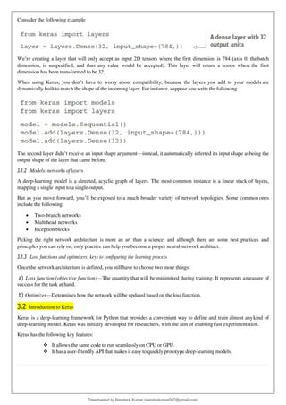
Consider the following example
We’re creating a layer that will only accept as input 2D tensors where the first dimension is 784 (axis 0, the batch
dimension, is unspecified, and thus any value would be accepted). This layer will return a tensor where the first
dimension has been transformed to be 32.
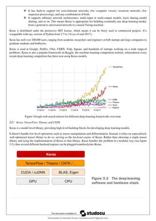
When using Keras, you don’t have to worry about compatibility, because the layers you add to your models are
dynamically built to match the shape of the incoming layer. For instance, suppose you write the following
The second layer didn’t receive an input shape argument—instead, it automatically inferred its input shape asbeing the
output shape of the layer that came before.
3.1.2 Models: networks of layers
A deep-learning model is a directed, acyclic graph of layers. The most common instance is a linear stack of layers,
mapping a single input to a single output.
But as you move forward, you’ll be exposed to a much broader variety of network topologies. Some common ones
include the following:
• Two-branch networks
• Multihead networks
• Inception blocks
Picking the right network architecture is more an art than a science; and although there are some best practices and
principles you can rely on, only practice can help you become a proper neural-network architect.
3.1.3 Loss functions and optimizers: keys to configuring the learning process
Once the network architecture is defined, you still have to choose two more things:
a) Loss function (objective function)—The quantity that will be minimized during training. It represents ameasure of
success for the task at hand.
b) Optimizer—Determines how the network will be updated based on the loss function.
3.2 Introduction to Keras
Keras is a deep-learning framework for Python that provides a convenient way to define and train almost anykind of
deep-learning model. Keras was initially developed for researchers, with the aim of enabling fast experimentation.
Keras has the following key features:
❖ It allows the same code to run seamlessly on CPU or GPU.
❖ It has a user-friendly API that makes it easy to quickly prototype deep-learning models.
lOMoARcPSD|45089905

❖ It has built-in support for convolutional networks (for computer vision), recurrent networks (for
sequence processing), and any combination of both.
❖ It supports arbitrary network architectures: multi-input or multi-output models, layer sharing,model
sharing, and so on. This means Keras is appropriate for building essentially any deep-learning model,
from a generative adversarial network to a neural Turing machine.
Keras is distributed under the permissive MIT license, which means it can be freely used in commercial projects. It’s
compatible with any version of Python from 2.7 to 3.6 (as of mid-2017).
Keras has well over 200,000 users, ranging from academic researchers and engineers at both startups and large companies to
graduate students and hobbyists.
Keras is used at Google, Netflix, Uber, CERN, Yelp, Square, and hundreds of startups working on a wide range of
problems. Keras is also a popular framework on Kaggle, the machine-learning competition website, wherealmost every
recent deep-learning competition has been won using Keras models.
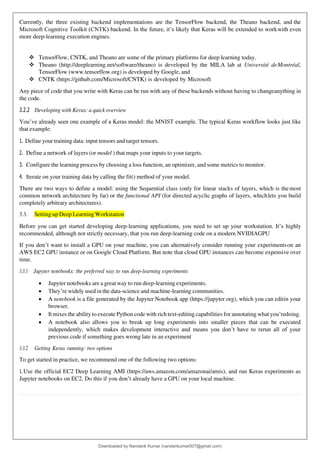
Figure: Google web search interest for different deep-learning frameworks over time
3.2.1 Keras, TensorFlow, Theano, and CNTK
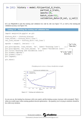
Keras is a model-level library, providing high-level building blocks for developing deep-learning models.
It doesn’t handle low-level operations such as tensor manipulation and differentiation. Instead, it relies on aspecialized,
well-optimized tensor library to do so, serving as the backend engine of Keras. Rather than choosing a single tensor
library and tying the implementation of Keras to that library, Keras handles the problem in a modular way (see figure
3.3); thus several different backend engines can be plugged seamlesslyinto Keras.
lOMoARcPSD|45089905

Currently, the three existing backend implementations are the TensorFlow backend, the Theano backend, and the
Microsoft Cognitive Toolkit (CNTK) backend. In the future, it’s likely that Keras will be extended to workwith even
more deep-learning execution engines.
❖ TensorFlow, CNTK, and Theano are some of the primary platforms for deep learning today.
❖ Theano (http://deeplearning.net/software/theano) is developed by the MILA lab at Université deMontréal,
TensorFlow (www.tensorflow.org) is developed by Google, and
❖ CNTK (https://github.com/Microsoft/CNTK) is developed by Microsoft
Any piece of code that you write with Keras can be run with any of these backends without having to changeanything in
the code.
3.2.2 Developing with Keras: a quick overview
You’ve already seen one example of a Keras model: the MNIST example. The typical Keras workflow looks just like
that example:
1. Define your training data: input tensors and target tensors.
2. Define a network of layers (or model ) that maps your inputs to your targets.
3. Configure the learning process by choosing a loss function, an optimizer, and some metrics to monitor.
4. Iterate on your training data by calling the fit() method of your model.
There are two ways to define a model: using the Sequential class (only for linear stacks of layers, which is themost
common network architecture by far) or the functional API (for directed acyclic graphs of layers, whichlets you build
completely arbitrary architectures).
3.3. Setting up Deep Learning Workstation
Before you can get started developing deep-learning applications, you need to set up your workstation. It’s highly
recommended, although not strictly necessary, that you run deep-learning code on a modern NVIDIAGPU
If you don’t want to install a GPU on your machine, you can alternatively consider running your experimentson an
AWS EC2 GPU instance or on Google Cloud Platform. But note that cloud GPU instances can become expensive over
time.
3.3.1 Jupyter notebooks: the preferred way to run deep-learning experiments
• Jupyter notebooks are a great way to run deep-learning experiments.
• They’re widely used in the data-science and machine-learning communities.
• A notebook is a file generated by the Jupyter Notebook app (https://jupyter.org), which you can editin your
browser.
• It mixes the ability to execute Python code with rich text-editing capabilities for annotating what you’redoing.
• A notebook also allows you to break up long experiments into smaller pieces that can be executed
independently, which makes development interactive and means you don’t have to rerun all of your
previous code if something goes wrong late in an experiment
3.3.2 Getting Keras running: two options
To get started in practice, we recommend one of the following two options:
1.Use the official EC2 Deep Learning AMI (https://aws.amazon.com/amazonai/amis), and run Keras experiments as
Jupyter notebooks on EC2. Do this if you don’t already have a GPU on your local machine.
lOMoARcPSD|45089905

2. Install everything from scratch on a local Unix workstation. You can then run either local Jupyter notebooks or a
regular Python codebase. Do this if you already have a high-end NVIDIA GPU.
3.3.3 Running deep-learning jobs in the cloud: pros and cons
There are many pros and cons to running deep-learning jobs in the cloud. Here are some of the most important ones:
Pros:
• Scalability: Cloud computing provides virtually unlimited scalability, so you can easily add or removeresources
as needed. This is essential for deep learning, as training models can be very demanding onresources.
• Cost-effectiveness: Cloud computing can be very cost-effective for deep learning, especially if you only need to use
the resources for a short period of time. You can also pay for the resources you use, soyou're not wasting money
on unused capacity.
• Ease of use: Cloud computing platforms make it easy to set up and run deep-learning jobs. Many platforms
provide pre-configured machine learning environments, so you don't have to worry about setting up the
infrastructure yourself.
• Collaboration: Cloud computing makes it easy to collaborate on deep learning projects. You can sharedata and
models with other team members, and you can also run jobs on multiple machines in parallel.
• Security: Cloud computing providers offer a high level of security for your data. Your data is encryptedin transit
and at rest, and you can control who has access to it.
Cons:
• Latency: There can be some latency when running deep-learning jobs in the cloud, as the data has totravel to
and from the cloud servers. This can be a problem for real-time applications.
• Vendor lock-in: If you choose to use a particular cloud provider, you may become locked in to their platform.
This can make it difficult to switch providers if you're not happy with their services.
• Complexity: Cloud computing can be complex, especially if you're not familiar with it. There are a lot of
different services and features to choose from, and it can be difficult to know which ones are rightfor you.
3.3.4 What is the best GPU for deep learning?
If you’re going to buy a GPU, which one should you choose? The first thing to note is that it must be an NVIDIA
GPU. NVIDIA is the only graphics computing company that has invested heavily in deep learning sofar, and modern
deep-learning frameworks can only run on NVIDIA cards
lOMoARcPSD|45089905

3.4. Classifying Movie Reviews: Binary Classification
Two-class classification, or binary classification, may be the most widely applied kind of machine-learning problem.
In this example, you’ll learn to classify movie reviews as positive or negative, based on the text content of the reviews.
3.4.1 The IMDB dataset
You’ll work with the IMDB dataset: a set of 50,000 highly polarized reviews from the Internet Movie Database.
They’re split into 25,000 reviews for training and 25,000 reviews for testing, each set consisting of50% negative and
50% positive reviews.
The argument num_words=10000 means you’ll only keep the top 10,000 most frequently occurring words inthe training
data. Rare words will be discarded. This allows you to work with vector data of manageable size
The variables train_data and test_data are lists of reviews; each review is a list of word indices (encoding asequence of
words). train_labels and test_labels are lists of 0s and 1s, where 0 stands for negative and 1 standsfor positive:
Because you’re restricting yourself to the top 10,000 most frequent words, no word index will exceed 10,000:
>>> max([max(sequence) for sequence in train_data])output:
9999
For kicks, here’s how you can quickly decode one of these reviews back to English words:
lOMoARcPSD|45089905

3.4.2 Preparing the data
You can’t feed lists of integers into a neural network. You have to turn your lists into tensors. There are twoways to do
that:
1. Pad your lists so that they all have the same length, turn them into an integer tensor of shape (samples,
word_indices), and then use as the first layer in your network a layer capable of handling such integer tensors (the
Embedding layer, which we’ll cover in detail later in the book).
2. One-hot encode your lists to turn them into vectors of 0s and 1s. This would mean, for instance, turning the
sequence [3, 5] into a 10,000-dimensional vector that would be all 0s except for indices 3 and 5, whichwould be 1s.
Then you could use as the first layer in your network a Dense layer, capable of handling floating-point vector data.
Let’s go with the latter solution to vectorize the data, which you’ll do manually for maximum clarity
Here’s what the samples look like now:
>>> x_train[0]
array([ 0., 1., 1., ..., 0., 0., 0.])
You should also vectorize your labels, which is straightforward:
y_train = np.asarray(train_labels).astype('float32')y_test
= np.asarray(test_labels).astype('float32')
3.4.3 Building your network
The input data is vectors, and the labels are scalars (1s and 0s): this is the easiest setup you’ll ever encounter.A type of
network that performs well on such a problem is a simple stack of fully connected (Dense) layers with relu activations:
Dense(16, activation='relu').
lOMoARcPSD|45089905

Finally, you need to choose a loss function and an optimizer. Because you’re facing a binary classification problem
and the output of your network is a probability (you end your network with a single-unit layer with a sigmoid
activation), it’s best to use the binary_crossentropy loss. It isn’t the only viable choice: you could use, for instance,
mean_squared_error. But crossentropy is usually the best choice when you’re dealing with models that output
probabilities.
3.4.4 Validating your approach
In order to monitor during training the accuracy of the model on data it has never seen before, you’ll createa validation
set by setting apart 10,000 samples from the original training data
You’ll now train the model for 20 epochs (20 iterations over all samples in the x_train and y_train tensors), inmini-
batches of 512 samples. At the same time, you’ll monitor loss and accuracy on the 10,000 samples thatyou set apart.
You do so by passing the validation data as the validation_data argument.
lOMoARcPSD|45089905

let’s use Matplotlib to plot the training and validation loss side by side (see figure 3.7), as well as the training and
validation accuracy (see figure 3.8).
As you can see, the training loss decreases with every epoch, and the training accuracy increases with everyepoch. That’s
what you would expect when running gradient descent optimization—the quantity you’re trying to minimize should be
less with every iteration.
lOMoARcPSD|45089905

3.5. Classifying newswires: Multiclass Classification
In this example, we will build a model to classify Reuters newswires into 46 mutually exclusive topics. Becausewe have
many classes, this problem is an instance of multiclass classification; and because each data point should be classified
into only one category, the problem is more specifically an instance of single-label, multiclass classification. If each
data point could belong to multiple categories (in this case, topics), you’d be facing a multilabel, multiclass
classification problem.
Reuters dataset
We will work with the Reuters dataset, a set of short newswires and their topics, published by Reuters in 1986. It’s a simple,
widely used toy dataset for text classification. There are 46 different topics; some topics are more represented than others,
but each topic has at least 10 examples in the training set. Like IMDB and MNIST, the Reuters dataset comes packaged as
part of Keras.
2.
3.
lOMoARcPSD|45089905

4. Data Prep
vectorize the input data
def vectorize_sequences(sequences, dimension=10000):results
= np.zeros((len(sequences), dimension))
for i, sequence in enumerate(sequences): results[i,
sequence] = 1.
return results
x_train = vectorize_sequences(train_data)#1 x_test =
vectorize_sequences(test_data)#2
1. Verctorize training data
2. Vencotrize testing data
vectorize the label with the exact same code as in the previous example. def
to_one_hot(labels, dimension=46):
results = np.zeros((len(labels), dimension))for i,
label in enumerate(labels):
results[i, label] = 1.
return results
one_hot_train_labels = to_one_hot(train_labels)#1
one_hot_test_labels = to_one_hot(test_labels)#2
1. Verctorize training labels
2. Vencotrize testing labels
Note that there is a built-in way to do this in Keras:
from tensorflow.keras.utils import to_categorical
one_hot_train_labels = to_categorical(train_labels)
one_hot_test_labels = to_categorical(test_labels)
5. Building the model
This topic-classification problem looks similar to the previous movie-review classification: in both cases, weare trying
to classify short snippets of text. But there is a new constraint here: the number of output classes has gone from 2 to 46. The
dimensionality of the output space is much larger.
In a stack of Dense layers like that we have been using, each layer can only access information present in theoutput of the
previous layer. If one layer drops some information relevant to the classification problem, thisinformation can never
be recovered by later layers: each layer can potentially become an information bottleneck. In the previous example, we
used 16-dimensional intermediate layers, but a 16-dimensional spacemay be too limited to learn to separate 46 different
classes: such small layers may act as information bottlenecks, permanently dropping relevant information. For this
reason we will use larger layers. Let’s go with 64 units.
lOMoARcPSD|45089905

Model Defination
model = keras.Sequential([
layers.Dense(64, activation='relu'),
layers.Dense(64, activation='relu'),
layers.Dense(46, activation='softmax')
])
Note about this architecture:
1. We end the model with a Dense layer of size 46. This means for each input sample, the network willoutput a
46-dimensional vector. Each entry in this vector (each dimension) will encode a different output class.
2. The last layer uses a softmax activation. You saw this pattern in the MNIST example. It means the model will
output a probability distribution over the 46 different output classes — for every input sample, the model will
produce a 46-dimensional output vector, where output[i] is the probability thatthe sample belongs to class i. The
46 scores will sum to 1.
3. The best loss function to use in this case is categorical_crossentropy. It measures the distance between two
probability distributions: here, between the probability distribution output by the model and the true
distribution of the labels. By minimizing the distance between these two distributions, you trainthe model to
output something as close as possible to the true labels.
6. Compile the model
model.compile(optimizer='rmsprop',
loss='categorical_crossentropy',
metrics=['accuracy'])
Validation of the approach
Let’s set apart 1,000 samples in the training data to use as a validation set.x_val =
x_train[:1000]
partial_x_train = x_train[1000:] y_val =
one_hot_train_labels[:1000]
partial_y_train = one_hot_train_labels[1000:]let’s
train the model for 20 epochs.
Training the model
history = model.fit(partial_x_train,
partial_y_train, epochs=20,
batch_size=512,
validation_data=(x_val, y_val))
lOMoARcPSD|45089905

Epoch 1/20
16/16 [==============================]
0.4079 - val_loss: 1.7132 - val_accuracy: 0.6440
- 2s 81ms/step - loss: 3.1029 - accuracy:
Epoch 2/20
16/16 [==============================]
Epoch 3/20
16/16 [==============================]
Epoch 4/20
16/16 [==============================]
Epoch 5/20
16/16 [==============================]
Epoch 6/20
16/16 [==============================] - 1s 37ms/step - loss: 0.5237 - accuracy:
Epoch 7/20
0.9160 - val_loss: 0.8765 - val_accuracy: 0.8140Epoch
8/20
16/16 [==============================]
Epoch 9/20
16/16 [==============================]
Epoch 10/20
16/16 [==============================]
Epoch 11/20
16/16 [==============================]
Epoch 12/20
Epoch 13/20
lOMoARcPSD|45089905

Epoch 14/20
16/16 [==============================]
Epoch 15/20
16/16 [==============================]
Epoch 16/20
16/16 [==============================]
Epoch 17/20
16/16 [==============================]
Epoch 18/20
16/16 [==============================]
Epoch 19/20
16/16 [==============================]
Epoch 20/20
7. Plotting the training and validation loss
loss = history.history['loss']
val_loss = history.history['val_loss']epochs =
range(1, len(loss) + 1)
plt.plot(epochs, loss, 'bo', label='Training loss')
plt.plot(epochs, val_loss, 'r', label='Validation loss')
plt.title('Training and validation loss') plt.xlabel('Epochs')
plt.ylabel('Loss')
plt.legend() plt.show()
lOMoARcPSD|45089905

lOMoARcPSD|45089905

unit-iii-deep-learningunit-iii-deep-learning.pdf

More Related Content

Similar to unit-iii-deep-learningunit-iii-deep-learning.pdf

More from nandan543979

Recently uploaded

unit-iii-deep-learningunit-iii-deep-learning.pdf