
![What is a Computation Graph?
import tensorflow as tf
matrix1 = tf.constant([[3., 3.]])
matrix2 = tf.constant([[2.],[2.]])
product = tf.matmul(matrix1, matrix2)
with tf.Session() as sess:
result = sess.run([product])
print(result)](https://image.slidesharecdn.com/gettingstartedwithkerasandtensorflow-stampedeconaisummit2017-171030121044/75/Getting-Started-with-Keras-and-TensorFlow-StampedeCon-AI-Summit-2017-10-2048.jpg)
![Computation Graph with Variables
import tensorflow as tf
sess = tf.InteractiveSession()
x = tf.Variable([1.0, 2.0])
a = tf.constant([3.0, 3.0])
x.initializer.run()
sub = tf.subtract(x, a)
print(sub.eval())
# ==> [-2. -1.]
sess.run(x.assign([4.0, 6.0]))
print(sub.eval())
# ==> [1. 3.]](https://image.slidesharecdn.com/gettingstartedwithkerasandtensorflow-stampedeconaisummit2017-171030121044/75/Getting-Started-with-Keras-and-TensorFlow-StampedeCon-AI-Summit-2017-11-2048.jpg)
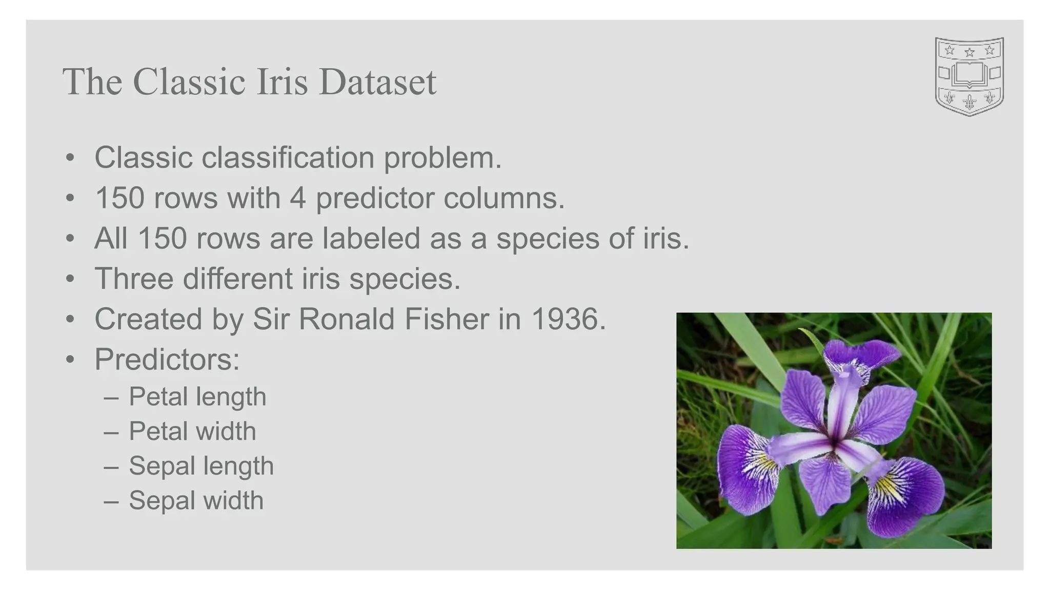
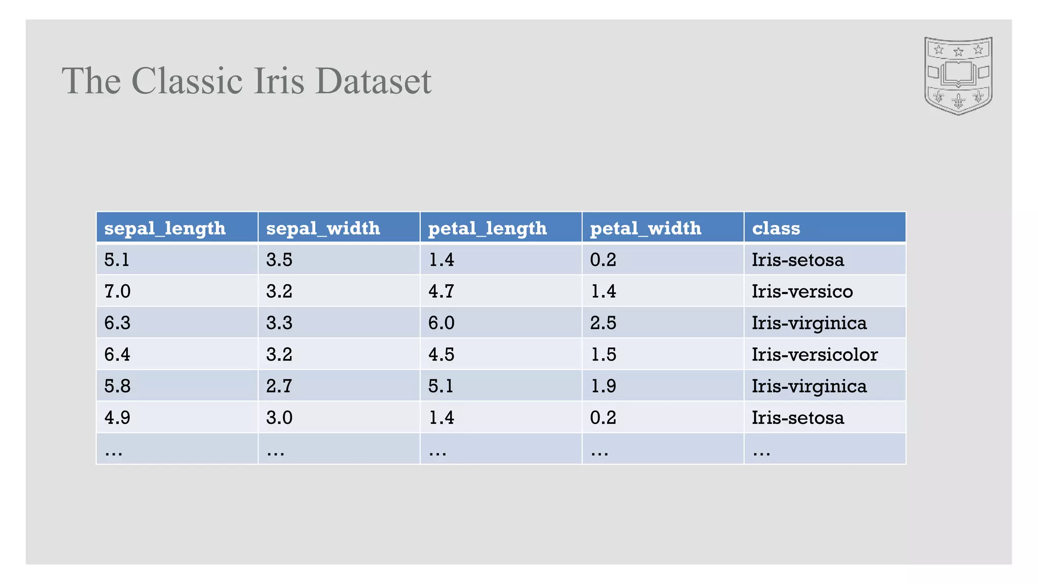
![Keras Classification: Load and Train/Test Split
path = "./data/"
filename = os.path.join(path,"iris.csv")
df = pd.read_csv(filename,na_values=['NA','?'])
species = encode_text_index(df,"species")
x,y = to_xy(df,"species")
# Split into train/test
x_train, x_test, y_train, y_test = train_test_split(
x, y, test_size=0.25, random_state=42)](https://image.slidesharecdn.com/gettingstartedwithkerasandtensorflow-stampedeconaisummit2017-171030121044/75/Getting-Started-with-Keras-and-TensorFlow-StampedeCon-AI-Summit-2017-31-2048.jpg)
![Keras Classification: Build NN and Fit
model = Sequential()
model.add(Dense(10, input_dim=x.shape[1],
kernel_initializer='normal', activation='relu'))
model.add(Dense(1, kernel_initializer='normal'))
model.add(Dense(y.shape[1],activation='softmax'))
model.compile(loss='categorical_crossentropy', optimizer='adam')
monitor = EarlyStopping(monitor='val_loss', min_delta=1e-3,
patience=5, verbose=1, mode='auto')
model.fit(x,y,validation_data=(x_test,y_test),callbacks=[monitor],ve
rbose=2,epochs=1000)](https://image.slidesharecdn.com/gettingstartedwithkerasandtensorflow-stampedeconaisummit2017-171030121044/75/Getting-Started-with-Keras-and-TensorFlow-StampedeCon-AI-Summit-2017-32-2048.jpg)
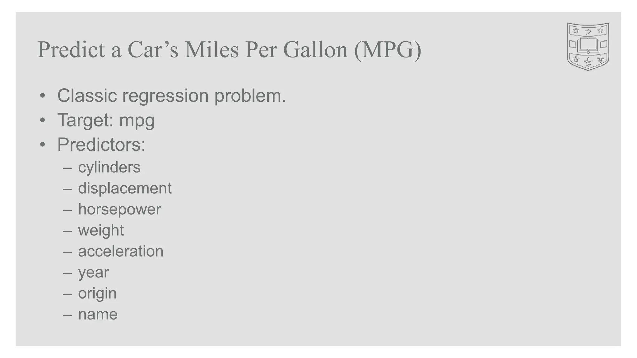
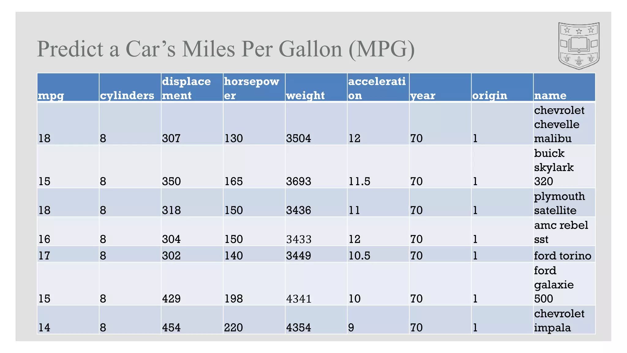
![Keras Regression: Load and Train/Test Split
path = "./data/"
filename_read = os.path.join(path,"auto-mpg.csv")
df = pd.read_csv(filename_read,na_values=['NA','?'])
cars = df['name']
df.drop('name',1,inplace=True)
missing_median(df, 'horsepower')
x,y = to_xy(df,"mpg")](https://image.slidesharecdn.com/gettingstartedwithkerasandtensorflow-stampedeconaisummit2017-171030121044/75/Getting-Started-with-Keras-and-TensorFlow-StampedeCon-AI-Summit-2017-38-2048.jpg)
![Keras Regression: Build and Fit
model = Sequential()
model.add(Dense(10, input_dim=x.shape[1],
kernel_initializer='normal', activation='relu'))
model.add(Dense(1, kernel_initializer='normal'))
model.compile(loss='mean_squared_error', optimizer='adam')
monitor = EarlyStopping(monitor='val_loss', min_delta=1e-3,
patience=5, verbose=1, mode='auto')
model.fit(x,y,validation_data=(x_test,y_test),callbacks=[monitor],ve
rbose=2,epochs=1000)](https://image.slidesharecdn.com/gettingstartedwithkerasandtensorflow-stampedeconaisummit2017-171030121044/75/Getting-Started-with-Keras-and-TensorFlow-StampedeCon-AI-Summit-2017-39-2048.jpg)


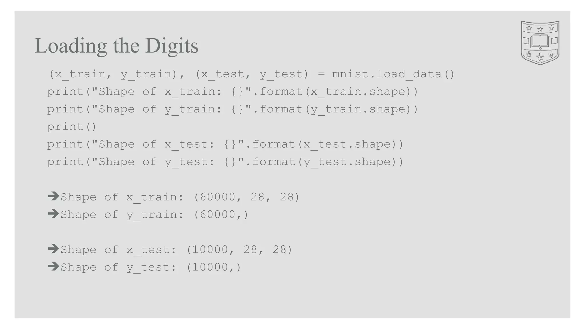
![Display a Digit
%matplotlib inline
import matplotlib.pyplot as plt
import numpy as np
digit = 101 # Change to choose new digit
a = x_train[digit]
plt.imshow(a, cmap='gray', interpolation='nearest')
print("Image (#{}): Which is digit '{}'".
format(digit,y_train[digit]))](https://image.slidesharecdn.com/gettingstartedwithkerasandtensorflow-stampedeconaisummit2017-171030121044/75/Getting-Started-with-Keras-and-TensorFlow-StampedeCon-AI-Summit-2017-50-2048.jpg)
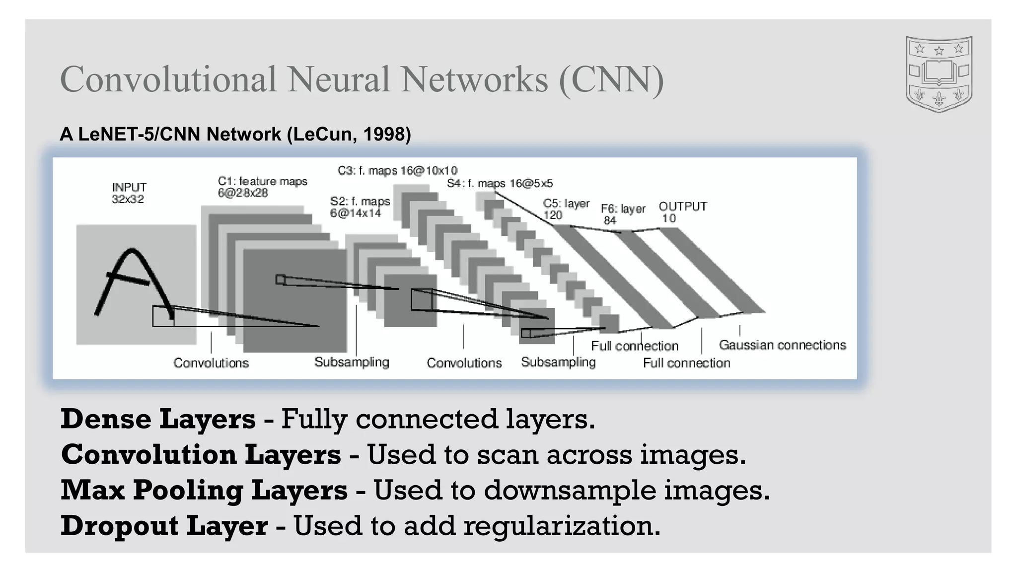
![Build the CNN Network
model = Sequential()
model.add(Conv2D(32, kernel_size=(3, 3),
activation='relu',
input_shape=input_shape))
model.add(Conv2D(64, (3, 3), activation='relu'))
model.add(MaxPooling2D(pool_size=(2, 2)))
model.add(Dropout(0.25))
model.add(Flatten())
model.add(Dense(128, activation='relu'))
model.add(Dropout(0.5))
model.add(Dense(num_classes, activation='softmax'))
model.compile(loss=keras.losses.categorical_crossentropy,
optimizer=keras.optimizers.Adadelta(),
metrics=['accuracy'])](https://image.slidesharecdn.com/gettingstartedwithkerasandtensorflow-stampedeconaisummit2017-171030121044/75/Getting-Started-with-Keras-and-TensorFlow-StampedeCon-AI-Summit-2017-51-2048.jpg)
![Fit and Evaluate
model.fit(x_train, y_train,
batch_size=batch_size,
epochs=epochs,
verbose=2,
validation_data=(x_test, y_test))
score = model.evaluate(x_test, y_test, verbose=0)
print('Test loss: {}'.format(score[0]))
print('Test accuracy: {}'.format(score[1]))
Test loss: 0.03047790436172363
Test accuracy: 0.9902
Elapsed time: 1:30:40.79 (for CPU, approx 30 min GPU)](https://image.slidesharecdn.com/gettingstartedwithkerasandtensorflow-stampedeconaisummit2017-171030121044/75/Getting-Started-with-Keras-and-TensorFlow-StampedeCon-AI-Summit-2017-52-2048.jpg)
![Sample Recurrent Data: Stock Price & Volume
x = [
[[32,1383],[41,2928],[39,8823],[20,1252],[15,1532]],
[[35,8272],[32,1383],[41,2928],[39,8823],[20,1252]],
[[37,2738],[35,8272],[32,1383],[41,2928],[39,8823]],
[[34,2845],[37,2738],[35,8272],[32,1383],[41,2928]],
[[32,2345],[34,2845],[37,2738],[35,8272],[32,1383]],
]
y = [
1,
-1,
0,
-1,
1
]](https://image.slidesharecdn.com/gettingstartedwithkerasandtensorflow-stampedeconaisummit2017-171030121044/75/Getting-Started-with-Keras-and-TensorFlow-StampedeCon-AI-Summit-2017-56-2048.jpg)
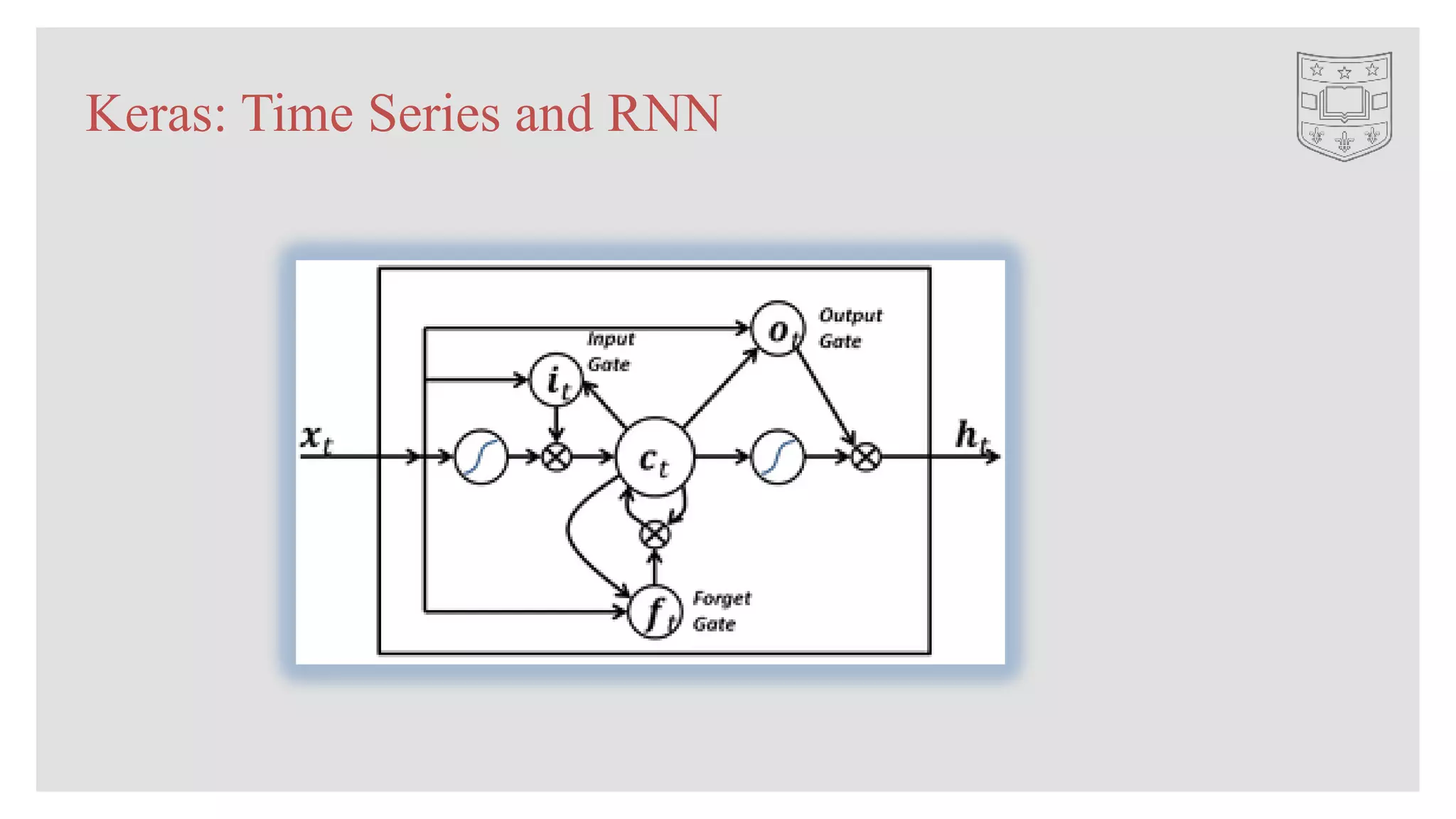
![LSTM Example
max_features = 4 # 0,1,2,3 (total of 4)
x = [
[[0],[1],[1],[0],[0],[0]],
[[0],[0],[0],[2],[2],[0]],
[[0],[0],[0],[0],[3],[3]],
[[0],[2],[2],[0],[0],[0]],
[[0],[0],[3],[3],[0],[0]],
[[0],[0],[0],[0],[1],[1]]
]
x = np.array(x,dtype=np.float32)
y = np.array([1,2,3,2,3,1],dtype=np.int32)](https://image.slidesharecdn.com/gettingstartedwithkerasandtensorflow-stampedeconaisummit2017-171030121044/75/Getting-Started-with-Keras-and-TensorFlow-StampedeCon-AI-Summit-2017-57-2048.jpg)
![Build a LSTM
model = Sequential()
model.add(LSTM(128, dropout=0.2, recurrent_dropout=0.2,
input_dim=1))
model.add(Dense(4, activation='sigmoid'))
model.compile(loss='binary_crossentropy',
optimizer='adam',
metrics=['accuracy'])](https://image.slidesharecdn.com/gettingstartedwithkerasandtensorflow-stampedeconaisummit2017-171030121044/75/Getting-Started-with-Keras-and-TensorFlow-StampedeCon-AI-Summit-2017-58-2048.jpg)
![Test the LSTM
def runit(model, inp):
inp = np.array(inp,dtype=np.float32)
pred = model.predict(inp)
return np.argmax(pred[0])
print( runit( model, [[[0],[0],[0],[0],[3],[3]]] ))
3
print( runit( model, [[[4],[4],[0],[0],[0],[0]]] ))
4](https://image.slidesharecdn.com/gettingstartedwithkerasandtensorflow-stampedeconaisummit2017-171030121044/75/Getting-Started-with-Keras-and-TensorFlow-StampedeCon-AI-Summit-2017-59-2048.jpg)


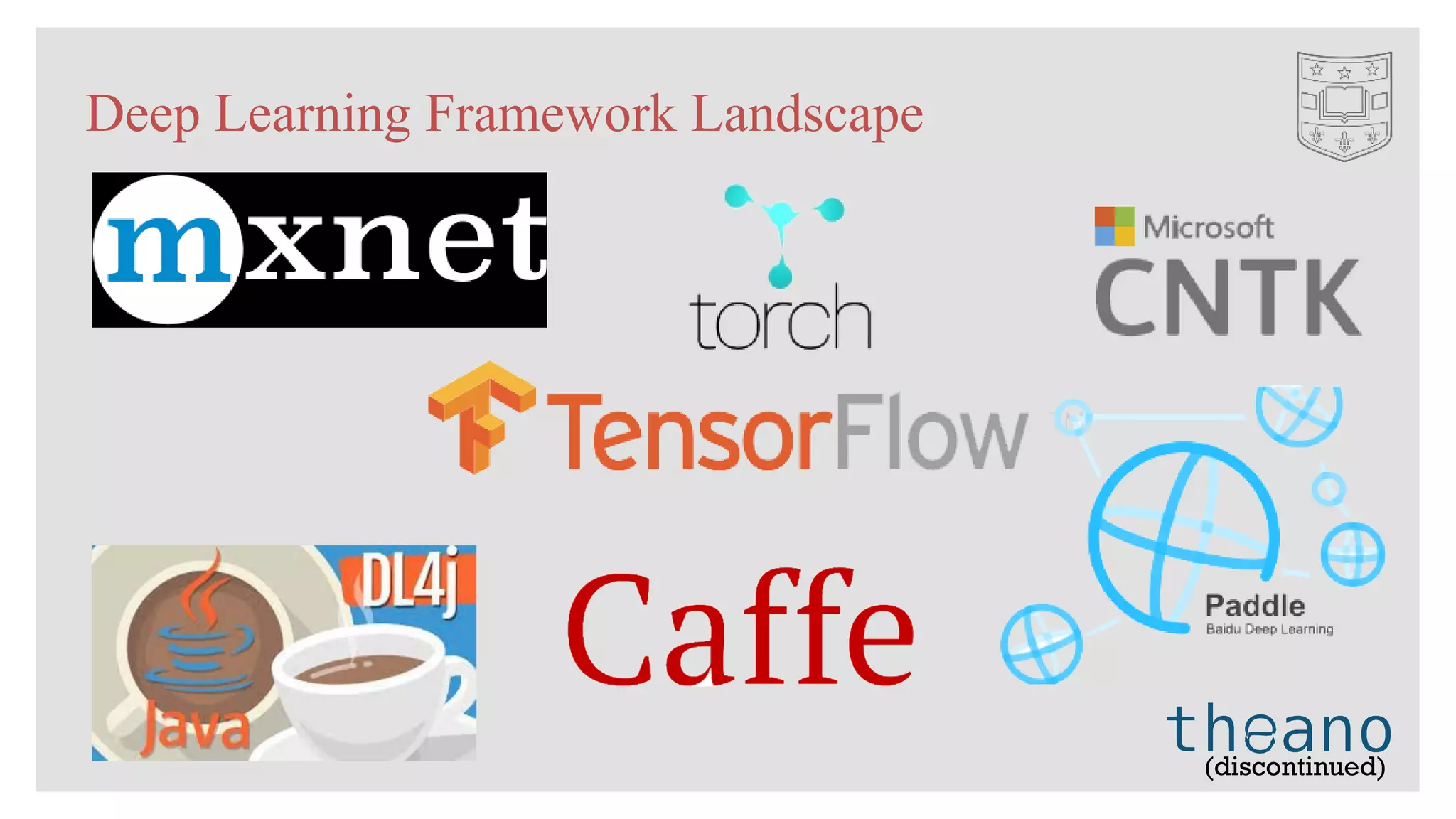
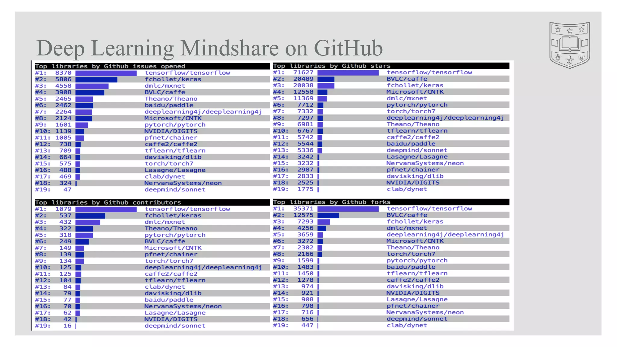
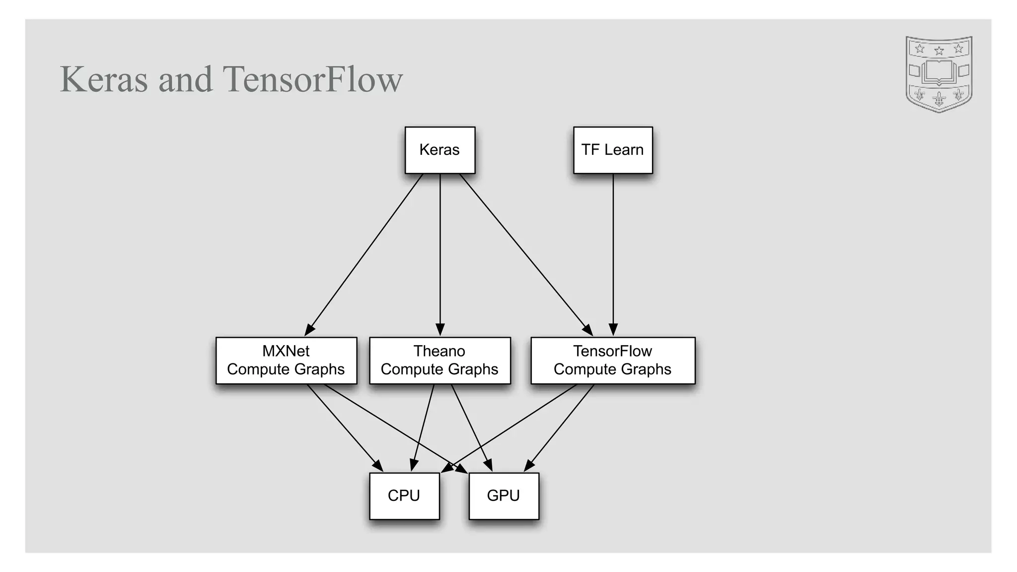
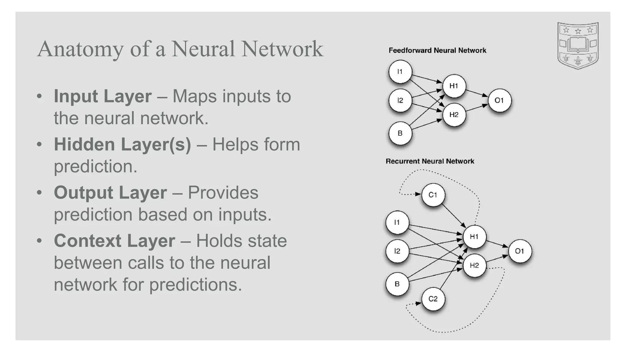
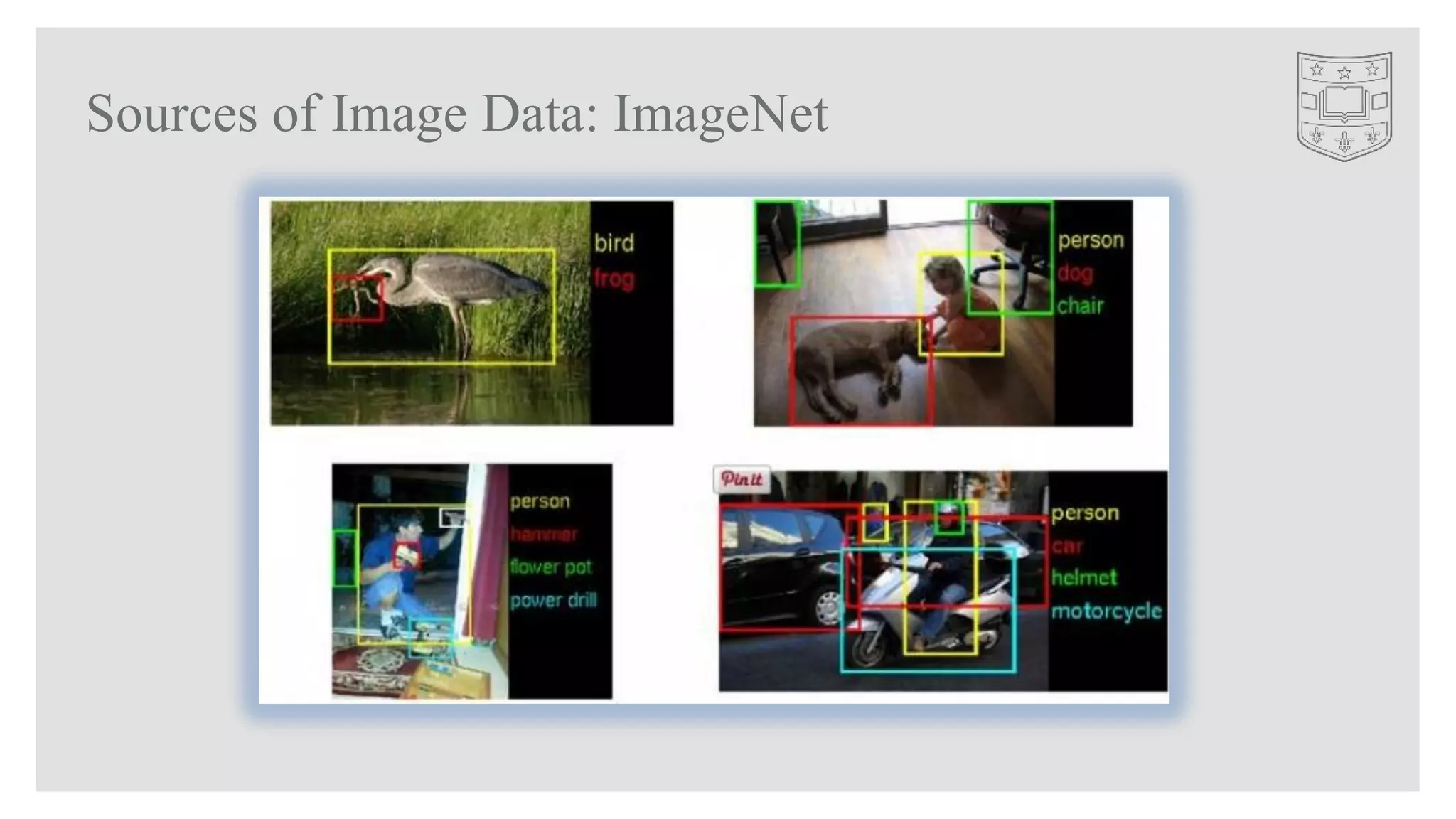
The document is a presentation on getting started with Keras and TensorFlow for deep learning, presented by Jeff Heaton at the AI Summit 2017. It covers topics including the deep learning framework landscape, various types of neural networks (CNNs, RNNs), classification, regression tasks, and practical implementations using Python tools like Keras and TensorFlow. Additionally, it provides code examples for building models and discusses the challenges of preparing real-world data for predictive modeling.


![Deep learning in python ommunic [CNN].pptx](https://cdn.slidesharecdn.com/ss_thumbnails/deeplearninginpythoncnn-251207084743-a5c807e1-thumbnail.jpg?width=640&height=640&fit=bounds)


![[DSC Europe 25] Ivan Peric - Intelligence Swarm Logic and Techno-Functional M...](https://cdn.slidesharecdn.com/ss_thumbnails/7my7c97fsduiccadgavw-2-251212103249-5a03f7c6-thumbnail.jpg?width=640&height=640&fit=bounds)


![[DSC Europe 25] Jovan Bogicevic - Legacy to AI-Driven Defense: Transforming D...](https://cdn.slidesharecdn.com/ss_thumbnails/rsarluadt563hntyfc8q-3-251211083849-3e7bc4c0-thumbnail.jpg?width=640&height=640&fit=bounds)
![[DSC Europe 25] Kaja Kandare - LLM as a judge.pptx](https://cdn.slidesharecdn.com/ss_thumbnails/arxyccaxsdsd1ba99wjw-7-251212104007-2b4e3f64-thumbnail.jpg?width=640&height=640&fit=bounds)
![[DSC Europe 25] Behzad Hosseini - AI Agents in the Wild: Deploying Models tha...](https://cdn.slidesharecdn.com/ss_thumbnails/3qtejajvsjqrzwfept2c-10-251212103250-7f2b1068-thumbnail.jpg?width=640&height=640&fit=bounds)
![[DSC Europe 25] Bassam Maharmeh - Artificial Intelligence: Opportunities and ...](https://cdn.slidesharecdn.com/ss_thumbnails/thhfmr2fqpawzj7hsjpg-5-251211083048-2c23204f-thumbnail.jpg?width=640&height=640&fit=bounds)
![[DSC Europe 25] Nikolay Burlutskiy - Best Practices for Building Enterprise M...](https://cdn.slidesharecdn.com/ss_thumbnails/uirvaiuvq8y1w8hzd9tx-7-251212103249-2619edb4-thumbnail.jpg?width=640&height=640&fit=bounds)
![[DSC Europe 25] Vladimir Jelic - The AI-Driven Security Shift From Reactive D...](https://cdn.slidesharecdn.com/ss_thumbnails/6g5gj25mtjwayniqem1t-6-251209104645-7a5a5fc6-thumbnail.jpg?width=640&height=640&fit=bounds)
![[DSC Europe 25] Jon Dajci - Bridging TradFi and DeFi: Building the Future of ...](https://cdn.slidesharecdn.com/ss_thumbnails/fqmhfvlbqhkihjvqvhmu-7-251211083849-6af7e325-thumbnail.jpg?width=640&height=640&fit=bounds)

![[DSC Europe 25] Branko Dzakula - From Defense to Attack: How AI Redefines Cyb...](https://cdn.slidesharecdn.com/ss_thumbnails/80bdzdxpr3ky2g0qvyk9-8-251211083048-ce5fc1ee-thumbnail.jpg?width=640&height=640&fit=bounds)
![[DSC Europe 25] Milan Zdravkovic - The road less traveled in District Heating...](https://cdn.slidesharecdn.com/ss_thumbnails/nfaboniqwsz4ucyctnmy-2-milan-zdravkovic-dsc2025-the-road-less-traveled-in-district-heating-operation-251208151905-f56388a5-thumbnail.jpg?width=640&height=640&fit=bounds)

![[DSC Europe 25] Marija Vlajkovic & Andrea Radonjanin - Integration of AI tool...](https://cdn.slidesharecdn.com/ss_thumbnails/qf1jrglttoc3bm8s3aop-final-integration-of-ai-tools-251208151905-394f3a6a-thumbnail.jpg?width=640&height=640&fit=bounds)
![[DSC Europe 25] Aleksandra Dragicevic - AI-Boosted Research in Healthcare: Fr...](https://cdn.slidesharecdn.com/ss_thumbnails/iqwngszurf2r7pi1lnnj-4-aleksandra-dragicevic-ad-dsc-europe-conference-20-251208151905-37c3238a-thumbnail.jpg?width=640&height=640&fit=bounds)
![[DSC Europe 25] Katherine Forrest - AI NOW: Understanding the Velocity of Cha...](https://cdn.slidesharecdn.com/ss_thumbnails/wvvbruqfrci0sfq9xwgb-4-251212104007-e5ad1987-thumbnail.jpg?width=640&height=640&fit=bounds)

![[DSC Europe 25] Sara Polak - The Ancient Operating System: What Archaeology T...](https://cdn.slidesharecdn.com/ss_thumbnails/3vch2p6tttdnwhsgazoz-3-sara-polak-smart-cities-251208152532-64404202-thumbnail.jpg?width=640&height=640&fit=bounds)