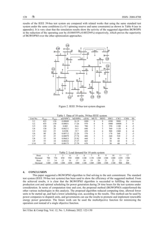
The article addresses the unit commitment problem in power systems to minimize production costs and optimize unit scheduling using a binary grey wolf optimizer based on particle swarm optimization (BGWOPSO) algorithm. It highlights the challenges in coordinating the operation of multiple generating units while adhering to various operational constraints, and presents simulation results from applying the method to a '39 bus IEEE test system.' The proposed approach outperforms other algorithms in minimizing costs and achieving efficient unit scheduling.

1. International Journal of Electrical and Computer Engineering (IJECE)
Vol. 12, No. 1, February 2022, pp. 122~130
ISSN: 2088-8708, DOI: 10.11591/ijece.v12i1.pp122-130  122
Journal homepage: http://ijece.iaescore.com
The optimal solution for unit commitment problem using binary
hybrid grey wolf optimizer
Ali Iqbal Abbas, Afaneen Anwer
Department of Electrical Engineering, University of Technology, Baghdad, Iraq
Article Info ABSTRACT
Article history:
Received Mar 22, 2021
Revised Jun 15, 2021
Accepted Jul 2, 2021
The aim of this work is to solve the unit commitment (UC) problem in
power systems by calculating minimum production cost for the power
generation and finding the best distribution of the generation among the
units (units scheduling) using binary grey wolf optimizer based on particle
swarm optimization (BGWOPSO) algorithm. The minimum production cost
calculating is based on using the quadratic programming method and
represents the global solution that must be arriving by the BGWOPSO
algorithm then appearing units status (on or off). The suggested method was
applied on “39 bus IEEE test systems”, the simulation results show the
effectiveness of the suggested method over other algorithms in terms of
minimizing of production cost and suggesting excellent scheduling of units.
Keywords:
Economic dispatch
Generation scheduling
Grey wolf optimizer
Particle swarm optimization
Unit commitment This is an open access article under the CC BY-SA license.
Corresponding Author:
Ali Iqbal Abbas
Department of Electrical Engineering, University of Technology
Baghdad, Iraq
Email: eee.19.14@grad.uotechnology.edu.iq
1. INTRODUCTION
Unit commitment is a significant issue in both the operation of electrical power systems and the
competitive electricity supply industry and market. It includes two decision-making processes: unit
scheduling and economic dispatch (ED). The generators scheduling process involves setting the status of
generating units every hour to be (ON or OFF) of the horizon planning while taking into account the
constraints of the units' minimum up and down-time. Process of determining the best power generation of
generation plants (units) to meet power demand and spinning reserve at every hour at the lowest production
cost within capacity unit limits using economic dispatch goals [1].
Because of load variation problem through the day, and for large power systems which contain
many plants or units, it is not suitable to operate all plants in time. So a method of coordination among these
plants and generating units must be adopted. The coordination involves in which units will be a start-up and
the sequence of operating units that must be connected to the network (i.e. ON) and which must be switched
OFF. Another problem must be solved that it produces electrical power with fulfilling demands in a
minimum cost [2].
Many methods have been used to solve the unit commitment (UC) problem as integer programming
[3], branch-and-bound methods [4], dynamic programming (DP) [5]-[8], mixed-integer programming [9],
and lagrangian relaxation methods (LR) [10], [11], and priority list method [12]. Also, there are many
optimization algorithms suggested to solve unit commitment as whale optimization-differential evolution and
genetic algorithm (WODEGA) [13], on mixed-integer programming formulations for the unit commitment
problem [14], solving unit commitment and economic load dispatch problems using modern optimization
algorithms [15], sested particle swarm optimization (PSO) [16], dynamic formulation of the unit commitment

2. Int J Elec & Comp Eng ISSN: 2088-8708 
The optimal solution for unit commitment problem using … (Ali Iqbal Abbas)
123
and economic dispatch problems [17]. In this paper the optimal UC solution based on binary grey wolf
optimizer based on particle swarm optimization (BGWOPSO) for (39 bus IEEE system with 10 units) has
been presented in discussion and the results compared with related works.
2. RESEARCH METHOD
Unit commitment (UC) issues are often used to assess which units must participate in dispatch
operations at particular times. The number of units, load capacity, startup cost, spinning reserve, and ramp
rate are all constraints that must be considered. The goal is to create a secure UC system that meets the
aforementioned constraints at a low total cost. According to their characteristics, power generating systems
may be listed as base-load, intermediate-load, or peak-load, so the main constraints can be listed as follows:
2.1. Constraints
In order to solve UC problem, the constraints must be satisfied which are imposed as operational
requirements. The constraints can be explained as following [1], [18]:
a. Power constraint
The sum of power generation of each generator at time t (𝑃𝑔𝑖
𝑡
) equal to demanded power:
∑ 𝑃𝑔𝑖
𝑡
= 𝑃𝐷
𝑡
𝑁𝑔
𝑖=1 (1)
where 𝑃𝐷
𝑡
represents active power which demanded at time t and 𝑁𝑔 number of generators.
b. Spinning reserve constraint
This term is used to characterize the total maximum active generated power from all units in the
system minus the current load demand. In other words, mathematically we can say:
∑ 𝑃𝑔𝑖
𝑁𝑔
𝑖=1 (Max) ≥ 𝑃𝐷
𝑡
+ 𝑃𝑅
𝑡
(2)
where Pgi(max) represents the maximum real power of the unit ( i), and 𝑃𝑅
𝑡
is the reserve of real power at time t.
c. Power limit constraints
𝑃𝑔𝑖(min) is is the minimum active power of unit i.
𝑃𝑔𝑖(min)≤ 𝑃𝑔𝑖
𝑡
≤ 𝑃𝑔𝑖(max) (3)
d. Minimum up time constraint
𝑇𝑖,𝑜𝑛
𝑡
is the number of hours that unit (i) is on till time t, and MUTi is the minimum uptime of unit (i).
𝑇𝑖,𝑜𝑛
𝑡
≥ 𝑀𝑈𝑇𝑖 (4)
e. Minimum down time constraint
𝑇𝑖,𝑜𝑓𝑓
𝑡
represents off hours of unit (i) till time t, and MDTi is the minimum downtime of unit (i).
𝑇𝑖,𝑜𝑓𝑓
𝑡
≥ 𝑀𝐷𝑇𝑖 (5)
In unit commitment, the priority list to make what unit is ON is based on the rate of the cost of full-
load (γ) for a unit which can define as the fuel cost divided on generated power at the maximum value of the
unit [1].
𝛾𝑖 =
𝑓𝑖
𝑃𝑔𝑖𝑚𝑎𝑥
(6)
𝛾𝑖 = a𝑖𝑃𝑔𝑖𝑚𝑎𝑥 + 𝑏𝑖 +
𝑐𝑖
𝑃𝑔𝑖𝑚𝑎𝑥
(7)
Where a unit that has 𝛾𝑖 the least with respect to other units will be prioritized to dispatch its power firstly.
The scheduling of units perhaps does not satisfy the constraint of spinning reserve. Therefore must solve this
violation that occurred. One approach that found to this purpose is depending on 𝛾𝑖 as following [1]:
a) At each time hour, find 𝛾𝑖 via (7) for each uncommitted unit at hour t, then sort them in an ascending
form.
b) Find the requirement of the spinning reserve at t by (2).

3.  ISSN: 2088-8708
Int J Elec & Comp Eng, Vol. 12, No. 1, February 2022: 122-130
124
c) In case the result occurred in point (2) achieves the constraint of spinning reserve, check t, if t < T, go to
point 1; otherwise, end this process. In the event point 2 is not achieved, one of the uncommitted units
must be committed that has the least 𝛾𝑖from point (1).
2.2. The economic dispatch
The main constraint of the operating system is the summation of the active output power of units
equal to power demand. The input to every unit, shown as fi, where fi refers to the cost rate of operation of
the unit (i) which is the fuel cost. The output of every unit, Pgi, is the active power generated by the ith unit.
The total cost represents the summation of the cost of each individual unit which mathematically denoted FT.
So the problem of economic dispatch is minimizing FT. The fuel cost fi of unit (i) at any interval time is a
function for the power generated of generating unit output Pgi [19].
(𝑓𝑖
𝑡
= 𝑐𝑖 + 𝑏𝑖𝑃𝑔𝑖 + 𝑎𝑖𝑃𝑔𝑖
2
) (8)
Where ai, bi, and ci are the fuel cost coefficients. The unit has incremental fuel cost (𝜆𝑖) which considered the
slope of the input-output curve and equal
𝜕𝑓𝑖
𝜕𝑃𝑔𝑖
= 𝜆𝑖. So, for the economical partition of load among units
within the plant, the norm is that all units must be operating at the same incremental fuel cost.
2.3. Hybrid grey wolf optimizer base on particle swarm optimization
2.3.1. Particle swarm optimization
Particle swarm optimization (PSO) is the algorithm presented by Kennedy and Eberhart [20]. This
theory was developed relying mainly on the intelligence of the swarm to do this advanced computational
procedure. In a swarm, every particle is considered a feasible solution to the optimization problem. The
movement of particles in space depends on the rules of flow. In the case of one of the particles discovering a
solution, the other particles will approach it. For all individuals, the values of fitness are estimated and that
will be optimized through the function of fitness. As a PSO is a tool of optimization, it provides an
exploration process in which residents constantly change their locations over time. Through investigation,
each particle maintains the best position it found, Pbest. In addition, among all the Pbest values gained the better
fitness is specific by one particle, which is known as the global best, known Gbest [21].
The position of the particle and velocity must be updated. Based on the fitness values the personal
location Pbest and global location Gbest are reconstituted as in (9)-(11) [1]:
𝑉𝑖
𝑡+1
= 𝑤𝑡
𝑉𝑖
𝑡
+ 𝑐1𝑟1
𝑡
(𝑃𝑏𝑒𝑠𝑡
𝑡
− 𝑥𝑖
𝑡
) + 𝑐2𝑟2
𝑡
(𝐺𝑏𝑒𝑠𝑡
𝑡
− 𝑥𝑖
𝑡
) (9)
𝑥𝑖
𝑡+1
= 𝑥𝑖
𝑡
+ 𝑉𝑖
𝑡+1
(10)
𝑤𝑡
: Inertia weight factor = 𝑤𝑚𝑎𝑥 −
𝑤𝑚𝑎𝑥−𝑤𝑚𝑖𝑛
𝐼𝑡𝑒𝑟𝑚𝑎𝑥
× 𝐼𝑡𝑒𝑟 (11)
where: “c1, c2: acceleration coefficient”, “x: the location of particle”, “r1, r2: Two numbers taken randomly
between 0 and 1”. “Vi
t
: The particle’s rapidity (velocity) in ith
dimension”. Also where “⍵max and ⍵min are the
initial and final weights and itermax is the maximum iteration number”.
2.3.2. Grey wolves optimizer (GWO)
This method relies on grey wolves' behavior in obtaining their food, as grey wolves are at the
topmost of predators [22]. The hierarchy of grey wolves is the leader in the herd is called alpha (α) and is
responsible for giving decisions. The second level is beta (β) wolves. The third and lower ranks of the pack
are delta (δ) and omega (w) respectively. Alpha is the fittest solution, both beta and delta will be the second
and third best solutions respectively [22]. Hunting prey begins first with the process of surrounding prey
(encircling), which can be modeled mathematically as in (12) and (13) [22]:
𝐷
⃗
⃗ = |𝐶. 𝑋𝑝(𝑘) − 𝑋𝑤(𝑘)| (12)
𝑋𝑤(𝑘 + 1) = 𝑋𝑝(𝑘) − 𝐴. 𝐷
⃗
⃗ (13)
where “k: the present iteration”, “𝐴 and 𝐷
⃗
⃗ : Coefficient vectors”, “ 𝑋𝑝: The position vector of prey”,
“𝑋𝑤: The position vector of the grey wolf”. It can calculate the vectors 𝐴 and 𝐶 as in (14) and (15):

4. Int J Elec & Comp Eng ISSN: 2088-8708 
The optimal solution for unit commitment problem using … (Ali Iqbal Abbas)
125
𝐴 = 2𝑎. 𝑟1
⃗⃗⃗ − 𝑎 (14)
𝐶 = 2 . 𝑟2
⃗⃗⃗ (15)
where throughout iterations components “𝑎 are decreased from 2 to 0 linearly” and “(𝑟1
⃗⃗⃗ , 𝑟2
⃗⃗⃗ ) are random
vectors between [0, 1]”.
Gray wolves can modify their position about the prey [23] and have the capability to distinguish the
prey's location. The hunting process is usually alpha-guided. To mathematically represent hunting behavior,
it suggests that alpha, beta, and delta have the best known probable site of the prey [22]. Therefore, the first
three optimal solutions it was obtained are kept to update their sites in the space proportional with the optimal
place [24], and the other solutions, including Omega solutions, are neglected [22]. These solutions can be
determined as in (16) [22].
𝐷𝛼
⃗⃗⃗⃗⃗ = |𝐶1
⃗⃗⃗⃗ . 𝑋𝛼
⃗⃗⃗⃗ (𝑘) − 𝑋|, 𝐷𝛽
⃗⃗⃗⃗ = |𝐶2
⃗⃗⃗⃗ . 𝑋𝛽
⃗⃗⃗⃗ (𝑘) − 𝑋|, 𝐷𝛿
⃗⃗⃗⃗ = |𝐶3
⃗⃗⃗⃗ . 𝑋𝛿
⃗⃗⃗⃗ (𝑘) − 𝑋| (16)
And by the following formulation can calculate the prey position vector with regard to (α, β, and δ)
respectively [22], [23]:
𝑥1
⃗⃗⃗ = 𝑋𝛼
⃗⃗⃗⃗ − 𝐴1
⃗⃗⃗⃗ . (𝐷𝛼
⃗⃗⃗⃗⃗ ) , 𝑥2
⃗⃗⃗⃗ = 𝑋𝛽
⃗⃗⃗⃗ − 𝐴2
⃗⃗⃗⃗ . (𝐷𝛽
⃗⃗⃗⃗ ), 𝑥3
⃗⃗⃗⃗ = 𝑋𝛿
⃗⃗⃗⃗ − 𝐴3
⃗⃗⃗⃗ . (𝐷𝛿
⃗⃗⃗⃗ ) (17)
where “𝑥1
⃗⃗⃗ , 𝑥2
⃗⃗⃗⃗ , 𝑥3
⃗⃗⃗⃗ are a three best solutions (wolves) in the pack at the given iteration k”. By taking the
average of 𝑥1
⃗⃗⃗ , 𝑥2
⃗⃗⃗⃗ , 𝑥3
⃗⃗⃗⃗ , it can calculate the best position as the formulation (18) [23].
𝑋(𝑘 + 1) =
𝑥1
⃗⃗⃗⃗ ,+𝑥2
⃗⃗⃗⃗ + 𝑥3
⃗⃗⃗⃗
3
(18)
As mentioned earlier 𝑎 are decreased from 2 to 0 linearly proportional with the number of iterations, the
algorithm has been updated by the (19) to calculate 𝑎 [24]:
𝑎 = 2 − 𝑘.
2
max 𝑖𝑡𝑒𝑟
(19)
where k: an iteration number, max iter: number of total iterations.
2.3.3. The hybridization
Thus, to hybridize the two meta-heuristic methods: GWO and PSO, the exploitation capability in
PSO and the exploration capability in GWO will be improved to get the strength of the two variables together
[25]. The first three optimal solutions are modified by the control the exploitation and exploration of the grey
wolves in the search area by inertia weight factor as in (20) [25]:
𝐷𝛼
⃗⃗⃗⃗⃗ = |𝐶1
⃗⃗⃗⃗ . 𝑋𝛼
⃗⃗⃗⃗ (𝑘) − 𝑤. 𝑋|, 𝐷𝛽
⃗⃗⃗⃗ = |𝐶2
⃗⃗⃗⃗ . 𝑋𝛽
⃗⃗⃗⃗ (𝑘) − 𝑤. 𝑋|, 𝐷𝛿
⃗⃗⃗⃗ = |𝐶3
⃗⃗⃗⃗ . 𝑋𝛿
⃗⃗⃗⃗ (𝑘) − 𝑤. 𝑋| (20)
Then velocity and position equations in (9) and (10) respectively in hybrid GWOPSO will be [25]:
𝑉𝑖
𝑡+1
= 𝑤𝑡
(𝑉𝑖
𝑡
+ 𝑐1𝑟1
𝑡
(𝑥1 − 𝑥𝑖
𝑡
) + 𝑐2𝑟2
𝑡
(𝑥2 − 𝑥𝑖
𝑡
) + 𝑐3𝑟3
𝑡
(𝑥3 − 𝑥𝑖
𝑡
) (21)
𝑥𝑖
𝑡+1
= 𝑥𝑖
𝑡
+ 𝑉𝑖
𝑡+1
(22)
2.4. Proposed method hybrid binary GWO based on PSO
Because of the algorithm hybrid GWOPSO is unable to solve the problem of feature selection since
it is binary problem by its nature, consequently, a binary version of the hybrid PSOGWO must be grown to
be appropriate for the feature selection problem [24]. Formulation (20) shown the modifying mechanism of
wolves be a function of three vectors' sites that is 𝑥1, 𝑥2; 𝑥3 and it promotes each wolf to the first three best
solutions, the updating of position in (18) can be upgraded into (23) [24]:
𝑥𝑑
𝑘+1
= { 1 𝑖𝑓 𝑠𝑖𝑔𝑚𝑜𝑖𝑑 (
𝑥1
⃗⃗⃗⃗ ,+𝑥2
⃗⃗⃗⃗ + 𝑥3
⃗⃗⃗⃗
3
) ≥ 𝑟𝑎𝑛𝑑
0 𝑜𝑡ℎ𝑒𝑟𝑤𝑖𝑠𝑒
(23)

5.  ISSN: 2088-8708
Int J Elec & Comp Eng, Vol. 12, No. 1, February 2022: 122-130
126
where “ 𝑥𝑑
𝑘+1
: the binary position which updated at kth iteration in dimension d” “rand: a random number
pulled from the uniform distribution ∈ [1,0]” and sigmoid (a) is denoted as in (24) [24]:
𝑠𝑖𝑔𝑚𝑜𝑖𝑑(𝑎) =
1
1+𝑒−10(𝑥−0.5) (24)
𝑥1, 𝑥2, 𝑥3 in (17) are updated and they are calculated by using formulation (25) [24]:
𝑥1
𝑑
= {1 𝑖𝑓 (𝑥𝛼
𝑑
+ 𝑏𝑠𝑡𝑒𝑝𝛼
𝑑
) ≥ 1
0 𝑜𝑡ℎ𝑒𝑟𝑤𝑖𝑠𝑒
𝑥2
𝑑
= {
1 𝑖𝑓 (𝑥𝛽
𝑑
+ 𝑏𝑠𝑡𝑒𝑝𝛽
𝑑
) ≥ 1
0 𝑜𝑡ℎ𝑒𝑟𝑤𝑖𝑠𝑒
(25)
𝑥3
𝑑
= {1 𝑖𝑓 (𝑥𝛿
𝑑
+ 𝑏𝑠𝑡𝑒𝑝𝛿
𝑑
) ≥ 1
0 𝑜𝑡ℎ𝑒𝑟𝑤𝑖𝑠𝑒
where 𝑥𝛼,𝛽,𝛿
𝑑
the position’s vector of (alpha, beta, and delta) wolves in dimension d.
𝑏𝑠𝑡𝑒𝑝𝛼
𝑑
: a binary step in dimension d that can be denoted as in (26) [24]:
𝑏𝑠𝑡𝑒𝑝𝛼,𝛽,𝛿
𝑑
= {
1 𝑖𝑓 𝑐𝑠𝑡𝑒𝑝𝛼,𝛽,𝛿
𝑑
≥ 𝑟𝑎𝑛𝑑
0 𝑜𝑡ℎ𝑒𝑟𝑤𝑖𝑠𝑒
(26)
where rand: a random number pulled from the uniform distribution ∈ [1, 0], (d): refers to dimension,
𝑐𝑠𝑡𝑒𝑝𝛼,𝛽,𝛿
𝑑
: Value of the d’s continuous and can be calculated by the next equation [24]:
𝑐𝑠𝑡𝑒𝑝𝛼,𝛽,𝛿
𝑑
=
1
1+𝑒
−10(𝐴1
𝑑𝐷𝛼,𝛽,𝛿
𝑑 −0.5)
(27)
Thus after update the best three solution positions through (25), in BGWOPSO the exploitation and
exploration are controlled by an inertia weight factor as in (28) [23]:
𝐷𝛼
⃗⃗⃗⃗⃗ = |𝐶1
⃗⃗⃗⃗ . 𝑋𝛼
⃗⃗⃗⃗ (𝑘) − 𝑤. 𝑋|, 𝐷𝛽
⃗⃗⃗⃗ = |𝐶2
⃗⃗⃗⃗ . 𝑋𝛽
⃗⃗⃗⃗ (𝑘) − 𝑤. 𝑋|, 𝐷𝛿
⃗⃗⃗⃗ = |𝐶3
⃗⃗⃗⃗ . 𝑋𝛿
⃗⃗⃗⃗ (𝑘) − 𝑤. 𝑋| (28)
Accordingly, the velocity and positions have been updated as in (29) [24]:
𝑉𝑖
𝑡+1
= 𝑤𝑡
(𝑉𝑖
𝑡
+ 𝑐1𝑟1
𝑡(𝑥1 − 𝑥𝑖
𝑡
) + 𝑐2𝑟2
𝑡(𝑥2 − 𝑥𝑖
𝑡
) + 𝑐3𝑟3
𝑡(𝑥3 − 𝑥𝑖
𝑡
) (29)
Note that in (29) the best three solutions 𝑥1, 𝑥2, 𝑥3 are updated according to (25) [24]:
𝑥𝑖
𝑡+1
= 𝑥𝑑
𝑘+1
+ 𝑉𝑖
𝑡+1
(30)
where 𝑥𝑑
𝑘+1
and 𝑉𝑖
𝑡+1
are calculated based on (23) and (29) respectively [24].
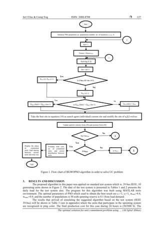
2.4.1. Unit commitment program structure using BGWOPSO
a. Initially, configured particles randomly and input other parameters as iteration number, c1, c2, and w.
within acceptable limits of generated power (pmin and pmax).
b. Calculate production cost (fi) and all ED requirements as shown in section (2.3).
c. Compare the present (fi) for each particle with Pbest. If the present (fi) is superior to Pbest, then this value is
Pbest otherwise Pbest same. Then determine Gbest among Pbest
d. Take the best site in (23) as search agent (individual) current site and modify the site of 𝛼, 𝛽, 𝛿 wolves
e. Take the site of alpha as the final site of the swarm and the alpha result as the best fitness.
f. Update the speed of each individual from (29).
g. Revise the position of individual xi
t
using (30).
h. If the iterations number arrives at the maximum number go to stride (9), else back to stride (3).
i. Determine the final cost of all combinations, division of power among the units, and trace the units'
scheduling.
Engender the best value of Gbest means that it is the best power that can be generated from each unit
with the lowest total generation cost. Figure 1 presents the above steps through flow chart.

6. Int J Elec & Comp Eng ISSN: 2088-8708 
The optimal solution for unit commitment problem using … (Ali Iqbal Abbas)
127
Figure 1. Flow chart of BGWOPSO algorithm in order to solve UC problem
3. RESULTS AND DISCUSSION
The proposed algorithm in this paper was applied on standard test system which is: 39 bus IEEE, 10
generating units shown in Figure 2. The date of the test system is presented in Tables 1 and 2 presents the
daily load for the test system also. The program for this algorithm was built using MATLAB tools
environment. The optimal parameters of PSO which used to obtain the best result are c1=1, c2=1, wmini=0.4,
wmaxi=0.9, and the number of populations is 50 with spinning reserve is 0.1 from load demand.
The results that arrived of simulating the suggested algorithm based on the test system (IEEE
39-bus) will be shown in Table 3 (see in appendix) where the units that participate in the operating system
are recognized in ping color. The final production cost for this case during 24 hours is (563940 $). The
No
Yes
Yes
No
No
Yes
No
Yes
2
Start
Initialize PSO parameters as: populations number, no. of iterations, c1,c2, w
Iter= 1
Fitness =fitness best
Iter= iter+1
ti=ti+1
is fi (pbest (i)) >pbest (i-1)
Pbest (i)= fi
Display the status
of committed
units, load sharing
between various
units and total cost
Pbest (i)= Pbest (i-1)
Update particle velocity from (29) and position from (30)
Iter=Itermax
Evaluate total cost,
no. of committed
units and power
distribution between
units
t=tmax
is Gbest (iter) > Gbest (iter-1) Gbest (iter) = Gbest
(iter)
Gbest (iter) = Gbest (iter-1)
2
End
Take the best site in equation (18) as search agent (individual) current site and modify the site of α,β,δ wolves
1
1
Solving E.D

7.  ISSN: 2088-8708
Int J Elec & Comp Eng, Vol. 12, No. 1, February 2022: 122-130
128
results of the IEEE 39-bus test system are compared with related works that using the same standard test
system under the same conditions (i.e 0.1 spinning reserve and same constraints) as shown in Table 4 (see in
appendix). It is very clear that the simulation results show the activity of the suggested algorithm BGWOPS
in the reduction of the operating cost by (0.046939%-0.003294%) respectively, which proves the superiority
of BGWOPSO over the other optimization approaches.
Figure 2. IEEE 39-bus test system diagram
Table 1. Data of 10 units, 39-bus IEEE system
Unit No. Pgimax Pgimin a($/MW2
) b($/MW) c($/h) MUTi MDTi HSCi CSCi CSHi ISi
U1 455 150 0.00048 16.19 1000 8 8 4500 9000 5 8
U2 455 150 0.00031 17.26 970 8 8 5000 10000 5 8
U3 130 20 0.002 16.6 700 5 5 550 1100 4 -5
U4 130 20 0.00211 16.5 680 5 5 560 1120 4 -5
U5 162 25 0.0398 19.7 450 6 6 900 1800 4 -6
U6 80 20 0.00712 22.26 370 3 3 170 340 2 -3
U7 85 25 0.00079 27.74 480 3 3 260 520 2 -3
U8 55 10 0.00413 25.92 660 1 1 30 60 0 -1
U9 55 10 0.00222 27.27 665 1 1 30 60 0 -1
U10 55 10 0.00173 27.79 670 1 1 30 60 0 -1
Table 2. Load demand for 10 units system
Hour 1 2 3 4 5 6 7 8 9 10 11 12
Demand 700 750 850 950 1000 1100 1150 1200 1300 1400 1450 1500
Hour 13 14 15 16 17 18 19 20 21 22 23 24
Demand 1400 1300 1200 1050 1000 1100 1200 1400 1300 1100 900 800
4. CONCLUSION
This paper suggested a BGWOPSO algorithm to find solving to the unit commitment. The standard
test system (IEEE 39-bus test systems) has been used to show the efficiency of the suggested method. From
the achieved results, it is clear that the BGWOPSO algorithm is succeeded to fulfilling the minimum
production cost and optimal scheduling for power generation during 24 time hours for the test systems under
consideration. In terms of computation time and cost, the proposed method (BGWOPSO) outperformed the
other various technologies in this analysis. The proposed algorithm reduced computing time, allowed fewer
units to be started up, and had a lower scheduling cost, according to the results. This method can be used by
power companies to dispatch units, and governments can use the results to promote and implement renewable
energy power generation. The future work can be used the multiobjective function for minimizing the
operation cost instead of a single objective function.

8. Int J Elec & Comp Eng ISSN: 2088-8708 
The optimal solution for unit commitment problem using … (Ali Iqbal Abbas)
129
APPENDIX
Table 3. Scheduling of generation and commitment of 10 units system by BGWOPSO
Generation scheduling
Hour Demand U1 U2 U3 U4 U5 U6 U7 U8 U9 U10
1 700 455 245 0 0 0 0 0 0 0 0
2 750 455 295 0 0 0 0 0 0 0 0
3 850 455 370 0 0 25 0 0 0 0 0
4 950 455 455 0 0 40 0 0 0 0 0
5 1000 455 390 0 130 25 0 0 0 0 0
6 1100 455 360 130 130 25 0 0 0 0 0
7 1150 455 410 130 130 25 0 0 0 0 0
8 1200 455 455 130 130 30 0 0 0 0 0
9 1300 455 455 130 130 85 20 25 0 0 0
10 1400 455 455 130 130 162 33 25 10 0 0
11 1450 455 455 130 130 162 73 25 10 10 0
12 1500 455 455 130 130 162 80 25 43 10 10
13 1400 455 455 130 130 162 33 25 10 0 0
14 1300 455 455 130 130 85 20 25 0 0 0
15 1200 455 455 130 130 30 0 0 0 0 0
16 1050 455 310 130 130 25 0 0 0 0 0
17 1000 455 260 130 130 25 0 0 0 0 0
18 1100 455 360 130 130 25 0 0 0 0 0
19 1200 455 455 130 130 30 0 0 0 0 0
20 1400 455 455 130 130 162 33 25 10 0 0
21 1300 455 455 130 130 85 20 25 0 0 0
22 1100 455 455 0 0 145 20 25 0 0 0
23 900 455 425 0 0 0 20 0 0 0 0
24 800 455 345 0 0 0 0 0 0 0 0
Units scheduling
Hour Demand U1 U2 U3 U4 U5 U6 U7 U8 U9 U10
1 700 1 1 0 0 0 0 0 0 0 0
2 750 1 1 0 0 0 0 0 0 0 0
3 850 1 1 0 0 1 0 0 0 0 0
4 950 1 1 0 0 1 0 0 0 0 0
5 1000 1 1 0 1 1 0 0 0 0 0
6 1100 1 1 1 1 1 0 0 0 0 0
7 1150 1 1 1 1 1 0 0 0 0 0
8 1200 1 1 1 1 1 0 0 0 0 0
9 1300 1 1 1 1 1 1 1 0 0 0
10 1400 1 1 1 1 1 1 1 1 0 0
11 1450 1 1 1 1 1 1 1 1 1 0
12 1500 1 1 1 1 1 1 1 1 1 1
13 1400 1 1 1 1 1 1 1 1 0 0
14 1300 1 1 1 1 1 1 1 0 0 0
15 1200 1 1 1 1 1 0 0 0 0 0
16 1050 1 1 1 1 1 0 0 0 0 0
17 1000 1 1 1 1 1 0 0 0 0 0
18 1100 1 1 1 1 1 0 0 0 0 0
19 1200 1 1 1 1 1 0 0 0 0 0
20 1400 1 1 1 1 1 1 1 1 0 0
21 1300 1 1 1 1 1 1 1 0 0 0
22 1100 1 1 0 0 1 1 1 0 0 0
23 900 1 1 0 0 0 1 0 0 0 0
24 800 1 1 0 0 0 0 0 0 0 0
The total cost= 563940 $
Table 4. Comparison total production cost between BGWOPSO and other approaches with
No. Method Best generation
cost ($)
Percentage of production cost
for BGWOPSO to another
algorithms
1 New Genetic Approach (NGA) [26] 591715 0.046939
2 Two Stage Genetic Algorithm (TSGA) [27] 568314.56 0.007694
3 GA [28] 565866 0.0034036
4 PSO-LR [29] 565835 0.003349
5 LR [28] 565828 0.003336
6 Improved DA-PSO [1] 565807.31 0.003299
7 Discrete Binary PSO [30] 565804 0.003294
8 Proposed method hybrid BGWOPSO 563940 -

9.  ISSN: 2088-8708
Int J Elec & Comp Eng, Vol. 12, No. 1, February 2022: 122-130
130
REFERENCES
[1] S. Khunkitti, N. R. Watson, R. Chatthaworn, S. Premrudeepreechacharn, and A. Siritaratiwat, “An improved DA-PSO
optimization approach for unit commitment problem,” Energies, vol. 12, 2019. doi: 10.3390/en12122335.
[2] S. Sivanagaraju and G. Sreenivasan, “Power system operation and control,” Pearson, 2009.
[3] K. W. Edwin, H. D. Kochs, and R. J. Taud, “Integer programming approach to the problem of optimal unit commitment with
probabilistic reserve determination,” IEEE Trans. Power Appar. Syst., vol. PAS-97, no. 6, pp. 2154–2166, 1978,
doi: 10.1109/TPAS.1978.354719.
[4] A. I. Cohen and M. Yoshimura, “A branch-and-bound algorithm for unit commitment,” IEEE Trans. Power Appar. Syst.,
vol. PAS-102, no. 2, pp. 444–451, 1983, doi: 10.1109/TPAS.1983.317714.
[5] C. K. Pang, G. B. Sheble, and F. Albuyeh, “Evaluation of dynamic programming based methods and multiple area representation
for thermal unit commitments,” IEEE Trans. Power Appar. Syst., vol. PAS-100, no. 3, pp. 1212–1218, 1981, doi:
10.1109/TPAS.1981.316592.
[6] W. L. Snyder, H. D. Powell, and J. C. Rayburn, “Dynamic programming approach to unit commitment,” IEEE Trans. Power
Syst., vol. 2, no. 2, pp. 339–348, 1987, doi: 10.1109/TPWRS.1987.4335130.
[7] C. C. Su and Y. Y. Hsu, “Fuzzy dynamic programming: An application to unit commitment,” IEEE Trans. Power Syst., vol. 6,
no. 3, pp. 1231–1237, 1991, doi: 10.1109/59.119271.
[8] P. K. Singhal and R. N. Sharma, “Dynamic programming approach for solving power generating unit commitment problem,” 2nd
Int. Conf. on Comp. and Commu. Tech., 2011, pp. 298–303, doi: 10.1109/ICCCT.2011.6075161.
[9] J. A. Muckstadt and R. C. Wilson, “An application of mixed-integer programming duality to scheduling thermal generating
systems,” IEEE Trans. Power Appar. Syst., vol. PAS-87, no. 12, pp. 1968–1978, 1968, doi: 10.1109/TPAS.1968.292156.
[10] F. Zhuang and F. D. Galiana, “Towards a more rigorous and practical unit commitment by lagrangian relaxation,” IEEE Trans.
Power Syst., vol. 3, no. 2, pp. 763–773, 1988, doi: 10.1109/59.192933.
[11] A. Merlin and P. Sandrin, “A new method for unit commitment at Electricite de France,” IEEE Trans. power Appar. Syst.,
vol. PAS-102, no. 5, pp. 1218–1225, 1983, doi: 10.1109/TPAS.1983.318063.
[12] G. B. Sheble, “Solution of the unit commitment problem by the method of unit periods,” IEEE Trans. Power Syst., vol. 5, no. 1,
pp. 257–260, 1990, doi: 10.1109/59.49114.
[13] A. Singh and A. Khamparia, “A hybrid whale optimization-differential evolution and genetic algorithm based approach to solve
unit commitment scheduling problem: WODEGA,” Sustain. Comput. Informatics Syst., vol. 28, 2020, doi:
10.1016/j.suscom.2020.100442.
[14] B. Knueven, J. Ostrowski, and J. P. Watson, “On mixed-integer programming formulations for the unit commitment problem,”
INFORMS J. Comput., vol. 32, no. 4, pp. 857–876, Sep. 2020, doi: 10.1287/ijoc.2019.0944.
[15] Z. G. Hassan, M. Ezzat, and A. Y. Abdelaziz, “Solving unit commitment and economic load dispatch problems using modern
optimization algorithms,” Int. J. Eng. Sci. Technol., vol. 9, no. 4, 2017, doi: 10.4314/ijest.v9i4.2.
[16] M. Farsadi, H. Hosseinnejad, and T. S. Dizaji, “Solving unit commitment and economic dispatch simultaneously considering
generator constraints by using nested PSO,” ELECO 2015 - 9th Int. Conf. Electr. Electron. Eng., 2016, pp. 493–499,
doi: 10.1109/ELECO.2015.7394478.
[17] M. Tuffaha and J. T. Gravdahl, “Dynamic formulation of the unit commitment and economic dispatch problems,” Proc. IEEE Int.
Conf. Ind. Technol., 2015, vol. 2015, pp. 1294–1298, doi: 10.1109/ICIT.2015.7125276.
[18] Y. Zhai, X. Liao, N. Mu, and J. Le, “A two-layer algorithm based on PSO for solving unit commitment problem,” Soft Comput.,
vol. 24, no. 12, pp. 9161–9178, 2020, doi: 10.1007/s00500-019-04445-x.
[19] A. J. Wood, B. F. Wollenberg, and G. B. Sheble, “Power generation, operation, and control,” 3rd ed, Wiley, New York, 2014.
[20] J. Kennedy and R. C. Eberhart, “Particle swarm optimization,” Proceedings of the IEEE International Conference on Neural
Networks, Perth, Australia, vol. 4, 1995, pp. 1942–1948.
[21] P. Sriyanyong and Y. H. Song, “Unit commitment using particle swarm optimization combined with lagrange relaxation,” IEEE
Power Eng. Soc. Gen. Meet., vol. 3, no. 6, pp. 2752–2759, 2005, doi: 10.1109/pes.2005.1489390.
[22] S. Mirjalili, S. M. Mirjalili, and A. Lewis, “Grey wolf optimizer,” Adv. Eng. Softw., vol. 69, pp. 46–61, 2014,
doi: 10.1016/j.advengsoft..12.007.
[23] V. K. Kamboj, “A novel hybrid PSO–GWO approach for unit commitment problem,” Neural Comput. Appl., vol. 27, no. 6,
pp. 1643–1655, 2016, doi: 10.1007/s00521-015-1962-4.
[24] Q. Al-Tashi, S. J. A. Kadir, H. M. Rais, S. Mirjalili, and H. Alhussian, “Binary optimization using hybrid grey wolf optimization
for feature selection,” IEEE Access, vol. 7, pp. 39496–39508, 2019, doi: 10.1109/ACCESS.2019.2906757.
[25] N. Singh and S. B. Singh, “Hybrid algorithm of particle swarm optimization and grey wolf optimizer for improving convergence
performance,” J. Appl. Math., vol. 2017, 2017, doi: 10.1155/2017/2030489.
[26] D. Ganguly, V. Sarkar, and J. Pal, “A new genetic approach for solving the unit commitment problem,” 2004 Int. Conf. Power
Syst. Technol. POWERCON 2004, vol. 1, pp. 542–547, 2004, doi: 10.1109/icpst.2004.1460054.
[27] A. S. Eldin, M. A. H. El-sayed, and H. K. M. Youssef, “A two-stage genetic based technique for the unit commitment
optimization problem,” 12th Int. Middle East Power Syst. Conf. 2008, pp. 425–430D.
[28] D. N. Simopoulos, S. D. Kavatza and C. D. Vournas, "Unit Commitment by an Enhanced Simulated Annealing Algorithm," 2006
IEEE PES Power Systems Conference and Exposition, 2006, pp. 193-201, doi: 10.1109/PSCE.2006.296296.
[29] H. H. Balci and J. F. Valenzuela, “Scheduling electric power generators using particle swarm optimization combined with the Lagrangian
relaxation method,” Int. J. Appl. Math. Comput. Sci., vol. 14, no. 3, pp. 411–421, 2004.
[30] Z. L. Gaing, “Discrete particle swarm optimization algorithm for unit commitment,” 2003 IEEE Power Eng. Soc. Gen. Meet.
Conf. Proc., vol. 1, pp. 418–424, 2003, doi: 10.1109/pes.2003.1267212.