1) The document describes an uncertain factor covariance model that accounts for uncertainty in risk forecasts. It models exposures, factor variances, and stock-specific effects as distributions rather than fixed values to represent forecast uncertainty.
2) The model allows for calculating the expected variance of a portfolio as well as the standard deviation, capturing uncertainty in the risk forecast. This enables more informed decision making that considers risks from imprecise estimates.
3) Applications discussed include portfolio optimization that maximizes risk-adjusted return while penalizing uncertainty, and pairs trading to select hedges with minimum uncertainty-adjusted risk. The model is aimed at improving forecasts and investment decisions by explicitly representing uncertainty.
Risk Parity with Uncertain Risk ContributionsAnish Shah
Risk parity is portfolio construction technique that, using risk alone, scales each part of a portfolio - e.g., stocks, bonds, currencies, commodities - so that its contribution to net portfolio risk matches its budgeted risk. Because contributions are measured using a point-estimate of covariance, the method is subject to problems of estimation error. Presented is a way to solve risk parity with covariance modeled as uncertain in order to achieve a weighting robust to changes in regime and hidden risks from misperceived hedging.
Having wide application outside of risk parity are the uncertain contributions calculated en route. Reporting a portfolio's "uncertain risk decomposition" reveals the range around numbers and, more important, the risks that arise from being wrong, e.g., market's going from invisible to the biggest latent risk in a seemingly beta-hedged long-short portfolio.
IFRS 13 CVA DVA FVA and the Implications for Hedge Accounting - By Quantifi a...Quantifi
International Financial Reporting Standard 13: fair value measurement (IFRS 13) was originally issued in May 2011 and applies to annual periods beginning on or after 1 January 2013. IFRS 13 provides a framework for determining fair value, clarifies the factors to be considered for estimating fair value and identifies key principles for estimating fair value. IFRS 13 facilitates preparers to apply, and users to better understand, the fair value measurements in financial statements, therefore helping improve consistency in the application of fair value measurement.
Measuring the behavioral component of financial fluctuaction. An analysis bas...SYRTO Project
Measuring the behavioral component of financial fluctuaction. An analysis based on the S&P 500 - Caporin M., Corazzini L., Costola M. - November 8, 2013.
ASSET 2013.
A Short Glimpse Intrododuction to Multi-Period Fuzzy Bond Imunization for Con...NABIH IBRAHIM BAWAZIR
A Short Glimpse Intrododuction to Multi-Period Fuzzy Bond Imunization for Construct Active Bond Portofolio, this paper is made to fullfill Fixed-Income securities mid semester exam
Impact of Valuation Adjustments (CVA, DVA, FVA, KVA) on Bank's Processes - An...Andrea Gigli
The talk hold in London on September 10th at the 5th Annual XVA Forum on Funding, Capital and Valuation. It covered some implications of Valuation Adjustments like CVA, DVA, FVA and KVA (XVAs) in the Pricing of Derivatives, Data Model Definition, Risk Management, Accounting, Trade Workflow processing.
Credit risks are calculated based on the borrowers’ overall ability to repay. Our objective was to use optimization in order to create a tool that approves or rejects loans to borrowers. We also used optimization to establish how much interest rate/credit will be extended to borrowers who were approved for a loan.
Creating an Explainable Machine Learning AlgorithmBill Fite
How to create an explainable scorecard model using machine learning to optimize its performance with results and insights from applying it to a stock picking problem.
Empirical Analysis of Bank Capital and New Regulatory Requirements for Risks ...Michael Jacobs, Jr.
We examine the impact of new supervisory standards for bank trading portfolios, additional capital requirements for liquidity risk and credit risk (the Incremental Risk Charge), introduced under Basel 2.5. We estimate risk measures under alternative assumptions on portfolio dynamics (constant level of risk vs. constant positions), rating systems (through-the-cycle vs. point-in-time), for different sectors (asset classes and industry groups), alternative credit risk frameworks (al-ternative dependency structures or factor models) and an extension to a Bayesian framework. We find a potentially material increase in capital requirements, above and beyond that concluded in the far-ranging impact studies conducted by the international supervisors utilizing the participation of a large sample of banks. Results indicate that capital charges are in general higher for either point-in-time ratings or constant portfolio dynamics, with this effect accentuated for financial or sovereign as compared to industrial sectors; and that regulatory is larger than economic capital for the latter, but not for the former sectors. A comparison of the single to a multi-factor credit models shows that capital estimates larger in the latter, and for the financial / sovereign by orders of magnitude vs. industrial or the Basel II model, and that there is less sensitivity of results across sectors and rating systems as compared with the single factor model. Furthermore, in a Bayesian experiment we find that the new requirements may introduce added uncertainty into risk measures as compared to existing approaches.
Fears in business operations are known as risks. They mainly affect external and international
relations and other business relations. In the event where operational risks are prominent, the
viability of a business in the future deteriorates and is a complete failure or crippling of the entire
business system. Risk aversion also takes into consideration proper analysis of future prospect of
a specific business before even making an ideal analysis of future prospect of a specific business
before engaging in capital investment
- See more at: http://www.customwritingservice.org/blog/risks-and-returns/
We review basic reserving methodologies for reserving general insurance like lag analysis and chain ladder. We then move forward to consider multiple stochastic loss reserving models in detail and show how they uncover more insights than basic reserving models.
AgendaComprehending risk when modeling investment (project) de.docxgalerussel59292
Agenda
Comprehending risk when modeling investment (project) decisions
Standalone Risk
Market Risk
1
1
Project Risk
Standalone Risk: Risk based on uncertainty of a projects cash flows
Sensitivity
Scenarios
Breakeven
Simulations
Market Risk: Risk of the project as seen by a well diversified investor
Beta
2
Sensitivity, Scenario, and Break-Even
Each allows us to look behind the NPV number to see how stable our estimates are.
Breakeven: sales required to breakeven
Accounting break-even: sales volume at which net income = 0
Cash break-even: sales volume at which operating cash flow = 0
Financial break-even: sales volume at which net present value = 0
Sensitivity: how sensitive a particular NPV calculation is to changes in an input variable holding all other assumptions are held constant
Scenario: examine impact on NPV given a confluence of factors
When working with spreadsheets, try to build your model so that you can adjust variables in a single cell and have the NPV calculations update accordingly.
3
3
Monte Carlo Simulation
A more sophisticated variation of the scenario analysis is Monte Carlo simulation.
In a Monte Carlo simulation, analysts specify a range or a distribution of potential outcomes for each of the model’s assumptions.
Pick a probability distribution for each input variable (units, price, variable costs, etc).
The computer program will pick a random value from each input variable, calculate the NPV and store the result. This is a trial.
Repeat the process many times, saving the input variables and the output (NPV).
End result: Probability distribution of NPV based on sample of simulated values.
4
Example
5
6
When a firm with both debt and equity invests in an asset similar to its existing assets (business), the WACC is the appropriate discount rate to use in NPV calculations.
In conglomerates, the WACC reflects the return that the firm must earn on average across all its assets to satisfy investors, but using the WACC to discount cash flows of a particular investment leads to mistakes.
Any project’s cost of capital depends on the use to which the capital is being put—not the source.
Therefore, it depends on the risk of the project and not the risk of the company.
When a firm invests in an asset that is different from its existing assets, it should look for pure-play firms to find the right discount rate.
6
Finding the Right Discount Rate
6
You are a financial analyst at General Electric and are preparing a cost of equity estimate for a project analysis using NPV:
CAPM = Risk Free Rate + Beta * Market Risk Premium
9.5% = 3.0% + 1.1 * 5.9%
Lines of Business
Financial Services
Power Generation
Aviation
Transportation
Health Care
Consumer Goods
When evaluating a new power generation investment for GE, which cost of capital should be used?
Capital Budgeting & Project Risk
7
Beta
1.8
0.6
1.2
1.3
0.8
1.1
7
17
Capital Budgeti.
Improving Returns from the Markowitz Model using GA- AnEmpirical Validation o...idescitation
Portfolio optimization is the task of allocating the investors capital among
different assets in such a way that the returns are maximized while at the same time, the
risk is minimized. The traditional model followed for portfolio optimization is the
Markowitz model [1], [2],[3]. Markowitz model, considering the ideal case of linear
constraints, can be solved using quadratic programming, however, in real-life scenario, the
presence of nonlinear constraints such as limits on the number of assets in the portfolio, the
constraints on budgetary allocation to each asset class, transaction costs and limits to the
maximum weightage that can be assigned to each asset in the portfolio etc., this problem
becomes increasingly computationally difficult to solve, ie NP-hard. Hence, soft computing
based approaches seem best suited for solving such a problem. An attempt has been made in
this study to use soft computing technique (specifically, Genetic Algorithms), to overcome
this issue. In this study, Genetic Algorithm (GA) has been used to optimize the parameters
of the Markowitz model such that overall portfolio returns are maximized with the standard
deviation of the returns being minimized at the same time. The proposed system is validated
by testing its ability to generate optimal stock portfolios with high returns and low standard
deviations with the assets drawn from the stocks traded on the Bombay Stock Exchange
(BSE). Results show that the proposed system is able to generate much better portfolios
when compared to the traditional Markowitz model.
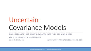
1. Uncertain
Covariance Models
RISK FORECASTS THAT KNOW HOW ACCURATE THEY ARE AND WHERE
NOV 9, 2015 QWAFAFEW SAN FRANCISCO
ANISH R. SHAH, CFA ANISHRS@INVESTMENTGRADEMODELING.COM
INVESTMENT GRADE MODELING, LLC INVESTMENTGRADEMODELING.COM
2. The Math of Uncertain Covariance
Straightforward … and not for a presentation
Shah, A. (2015). Uncertain Covariance Models
http://ssrn.com/abstract=2616109
Questions or comments, please email
AnishRS@InvestmentGradeModeling.com
INVESTMENT GRADE MODELING, LLC INVESTMENTGRADEMODELING.COM
3. Background: Why Care About
Covariance?
Notions of co-movement are needed to make decisions throughout the investment process
1. Estimating capital at risk and portfolio volatility
2. Hedging
3. Constructing and rebalancing portfolios through optimization
4. Algorithmic trading
5. Evaluating performance
6. Making sense of asset allocation
INVESTMENT GRADE MODELING, LLC INVESTMENTGRADEMODELING.COM
4. Background: Why Care About
Uncertainty?
1. Nothing is exactly known. Everything is a forecast
2. However, one can estimate the accuracy of individual numbers
Suppose two stocks have the same expected covariance against other securities
The first has been well-predicted in the past, the other not
Which is a safer hedge?
3. It’s imprudent to make decisions without considering accuracy
A fool, omitting accuracy from his objective, curses optimizers for taking numbers at face value
4. Relying on wrong numbers can cost you your shirt
under leverage
when you can be fired and have assets assigned to another manager
INVESTMENT GRADE MODELING, LLC INVESTMENTGRADEMODELING.COM
5. A Factor Covariance Model in Pictures
INVESTMENT GRADE MODELING, LLC INVESTMENTGRADEMODELING.COM
GOOG
Market
Risk Factors
Exposures
Stock-Specific
Effect
AAPL
GE
Growth-Value
Spread
Together these constitute a
model of how securities move –
jointly (winds and sails) and
independently (motors)
6. The Math of a Factor Covariance Model
1. Say a stock’s return is partly a function of pervasive factors, e.g. the return of the market and oil
𝑟𝐺𝑂𝑂𝐺 = ℎ 𝐺𝑂𝑂𝐺 𝑓 𝑚𝑘𝑡, 𝑓𝑜𝑖𝑙 + stuff assumed to be independent of the factors and other securities
2. Imagine linearly approximating this function
𝑟𝐺𝑂𝑂𝐺 ≈
𝜕ℎ 𝐺𝑂𝑂𝐺
𝜕𝑓 𝑚𝑘𝑡
𝑓 𝑚𝑘𝑡 +
𝜕ℎ 𝐺𝑂𝑂𝐺
𝜕𝑓 𝑜𝑖𝑙
𝑓𝑜𝑖𝑙 + constant + stuff
3. Model a stock’s variance as the variance of the approximation
𝑣𝑎𝑟 𝑟𝐺𝑂𝑂𝐺 ≈
𝜕ℎ 𝐺𝑂𝑂𝐺
𝜕𝑓 𝑚𝑘𝑡
𝜕ℎ 𝐺𝑂𝑂𝐺
𝜕𝑓 𝑜𝑖𝑙
exposures
sails
𝑣𝑎𝑟 𝑓 𝑚𝑘𝑡 𝑐𝑜𝑣 𝑓 𝑚𝑘𝑡, 𝑓𝑜𝑖𝑙
𝑐𝑜𝑣 𝑓 𝑚𝑘𝑡, 𝑓𝑜𝑖𝑙 𝑣𝑎𝑟 𝑓𝑜𝑖𝑙
factor covariance
how wind blows
𝜕ℎ 𝐺𝑂𝑂𝐺
𝜕𝑓 𝑚𝑘𝑡
𝜕ℎ 𝐺𝑂𝑂𝐺
𝜕𝑓 𝑜𝑖𝑙
exposures
sails
+ 𝑣𝑎𝑟 stuff
stock specific variance
size of motor
INVESTMENT GRADE MODELING, LLC INVESTMENTGRADEMODELING.COM
7. The Math of a Factor Covariance Model
4. Covariance between stocks is modeled as the covariance of their approximations
𝑐𝑜𝑣 𝑟𝐺𝑂𝑂𝐺, 𝑟𝐺𝐸 ≈
𝜕ℎ 𝐺𝑂𝑂𝐺
𝜕𝑓 𝑚𝑘𝑡
𝜕ℎ 𝐺𝑂𝑂𝐺
𝜕𝑓 𝑜𝑖𝑙
exposures
sails (𝐺𝑂𝑂𝐺)
𝑣𝑎𝑟 𝑓 𝑚𝑘𝑡 𝑐𝑜𝑣 𝑓 𝑚𝑘𝑡, 𝑓𝑜𝑖𝑙
𝑐𝑜𝑣 𝑓 𝑚𝑘𝑡, 𝑓𝑜𝑖𝑙 𝑣𝑎𝑟 𝑓𝑜𝑖𝑙
factor covariance
how wind blows
𝜕ℎ 𝐺𝐸
𝜕𝑓 𝑚𝑘𝑡
𝜕ℎ 𝐺𝐸
𝜕𝑓 𝑜𝑖𝑙
exposures
sails (𝐺𝐸)
Note: no motors here – they are assumed independent across stocks
5. Parts aren’t known but inferred, typically by regression, or by more sophisticated tools
6. Best is to forecast values over one’s horizon
INVESTMENT GRADE MODELING, LLC INVESTMENTGRADEMODELING.COM
8. INVESTMENT GRADE MODELING, LLC INVESTMENTGRADEMODELING.COM
GOOG
Uncertain Risk Factors
projected onto orthogonal directions
Uncertain
Exposures
Uncertain
Stock-Specific
Effect
Welcome to reality!
Nothing is known with certainty.
But some forecasts are believed
more accurate than others
A portfolio’s risk has – according
to beliefs – an expected value
and a variance
Good decisions come from
considering uncertainty explicitly.
Ignoring doesn’t make it go away
An Uncertain Factor Covariance Model
9. Uncertain Exposures
Beliefs about future exposure to the factors are communicated as Gaussian
◦ 𝒆 𝐺𝑂𝑂𝐺 ~ 𝑁 𝒆 𝐺𝑂𝑂𝐺, 𝛀 𝐺𝑂𝑂𝐺
◦ Exposures can be correlated across securities
◦ Estimates of mean and covariance come from the method to forecast exposures and historical accuracy
So, a portfolio’s exposures are also Gaussian
◦ This fact is used in the math to work out variance (from uncertainty) of portfolio return variance
INVESTMENT GRADE MODELING, LLC INVESTMENTGRADEMODELING.COM
10. Sidebar: E[β2] > (E[β])2
Ignoring Uncertainty Underestimates Risk
A CAPM flavored bare bones example to illustrate the idea:
◦ Stock’s return = market return × β
◦ Variance of stock’s return = market var × β2
Say β isn’t known exactly
◦ E[variance of stock’s return] = market var × E[β2]
= market var × (E2[β] + var[β] )
> market var × E2[β]
Ignoring uncertainty underestimates risk
◦ Note: this has nothing to do with aversion to uncertainty
INVESTMENT GRADE MODELING, LLC INVESTMENTGRADEMODELING.COM
“uncertainty correction”
11. Uncertain Factor Variances
Beliefs about the future factor variances are communicated as their mean and covariance
◦ Forecasts are the mean and covariance – according to uncertainty – of return variances
◦ Not Gaussian since variances ≥ 0
How the heck do you generate these?
Shah, A. (2014). Short-Term Risk and Adapting Covariance Models to Current Market Conditions
◦ http://ssrn.com/abstract=2501071
1. Forecast whatever you can, e.g. from VIX and cross-sectional returns, the volatility of S&P 500 daily
returns over the next 3 months will be 25% ± 5% annualized
2. The states of quantities measured by the risk model imply a configuration of factor variances
Since this inferred distribution of factor variances arises from predictions, it is a forecast
INVESTMENT GRADE MODELING, LLC INVESTMENTGRADEMODELING.COM
12. Adapting Infers Distribution
Of Factor Variances
INVESTMENT GRADE MODELING, LLC INVESTMENTGRADEMODELING.COM
SP
500
IBM
WM
OIL
1. Noisy variance forecasts via all manner
of Information sources
Implied vol, intraday price movement, news
and other big data, …
2. Imply a distribution on how the world is
3. An aside: this extends to the behavior of other securities
All risk forecasts are improved
JNJ
SB UX
FDX
13. Uncertain Stock-Specific Effects
Stock-specific effects (motors) are best regarded as both exposures (sails) and factors (wind)
1. A motor is like wind that affects just 1 stock
2. Its size is estimated with error like a sail
3. The average size of motors across securities varies over time
e.g. stock-specific effects can shrink as market volatility rises
Since it might depend on the variance of other factors, average size gets treated like one
Thus, uncertainty from stock-specific effects is captured using both types of uncertainty in the
preceding slides.
INVESTMENT GRADE MODELING, LLC INVESTMENTGRADEMODELING.COM
14. All Set with Machinery:
Uncertain Portfolio Variance
Math then yields for a portfolio
◦ expected variance
◦ standard deviation of variance
according to beliefs (estimates) about uncertainty in the pieces
◦ exposures
◦ factor variances
◦ stock-specific effects
Expectation and standard deviation are with respect to beliefs
◦ Not reality, but one’s best assessment of it
◦ “Given my beliefs, the portfolio’s tracking variance is E ± sd”
◦ What a person (or computer) needs to make good decisions from the information at hand
INVESTMENT GRADE MODELING, LLC INVESTMENTGRADEMODELING.COM
16. Portfolio Optimization: Uncertain Utility
Conventional
maxw U(w) = r(w) – λ × v(w) where r(w) = mean return, v(w) = variance of return
Uncertain
maxw O(w) = E[U(w)] – γ × stdev[U(w)]
var[U(w)] = var[r(w)] + λ2 var[v(w)] – 2 λ stdev[r(w)] stdev[v(w)] × ρw
ρw = cor[r(w), v(w)] for portfolio w, the correlation of uncertainty in mean and in variance
r(w) ~ N[wTμ, wTΣw] assume mean returns have Gaussian error
All pieces are known except ρw which, absent beliefs, can be set to 0
INVESTMENT GRADE MODELING, LLC INVESTMENTGRADEMODELING.COM
17. Portfolio Optimization:
Maximize Risk Adjusted Return
Risk-adjusted return ≡ portfolio alpha - ½ portfolio tracking variance
Say alpha is known exactly
Randomly pick 10 securities – ½ are eq wt benchmark, ½ are optimized into fully invested portfolio
Optimize under the following covariance models
Base conventional Bayesian 15 factor PCA model
Adapted base model adapted to forecasts of future market conditions
Uncertain[γ] adapted model with uncertainty information
maximize alpha - ½ [variance + γ stdev(variance)]
note: Uncertain[0] has uncertainty correction, but no penalty on uncertainty
Measure the shortfall in realized risk-adjusted return vs. the ideal (w/future covariance known)
Repeat the experiment 1000 times
INVESTMENT GRADE MODELING, LLC INVESTMENTGRADEMODELING.COM
18. Portfolio Optimization:
Maximize Risk Adjusted Return (cont)
INVESTMENT GRADE MODELING, LLC INVESTMENTGRADEMODELING.COM
-140
-120
-100
-80
-60
-40
-20
0
Base Adapted Uncertain[0] Uncertain[0.1] Uncertain[1] Uncertain[10]
RISKADJUSTEDRETURN
Shortfall in realized risk-adjusted return vs decision with future covariance known
10% 25% 50% 75% 90%
Considering uncertainty tames downside
without costing upside
2013-Jun-27 with a horizon of 20 trading days
percentile:
of the 1000 experiments
22. Pairs Trading
Improved via knowledge of uncertainty
◦ Feel bullish (or bearish) about one or several similar securities
◦ Have candidates you feel the opposite about
◦ Choose – from the two sets – the long-short pair with lowest uncertainty
penalized risk
◦ If you have explicit alpha forecasts, instead maximize uncertain utility
◦ Better risk control = safer leverage and more room to pursue alpha
A toy example, hedging with 3 securities
◦ AAPL is the reference security
◦ Every 11 trading days from 2012 through 2013, find the best 3 hedges
(ignoring stock-specific effects) from a universe of tech stocks and equal
weight-them
◦ Calculate the subsequent 10 day volatility of daily returns of long AAPL,
short the equal weighted
Model Avg 1 Day TE
Base 1.34
Uncertain[0] 1.13
Uncertain[0.5] 1.14
Uncertain[1] 1.13
Uncertain[100] 1.15
INVESTMENT GRADE MODELING, LLC INVESTMENTGRADEMODELING.COM
23. Investment Grade Modeling LLC
Uncertain Covariance Models
Run nightly in the cloud. Bloomberg BBGID or ticker
Built uniquely for each use
◦ Risk factors arise from one’s universe (e.g. only healthcare + tech, all US equities + commodity indices)
◦ .. and horizon (e.g. 1 day, 6 months) and return frequency (daily or weekly)
◦ Exposures (sails) are forecasts of the average over the horizon
◦ Factors volatilities (winds) and specific risks (motors) are adapted to forecasts of future volatility over
the horizon made from broad set of information
◦ Though I believe risk crowding is baloney: zero chance of crowding from others using an identical model
“Augmented” PCA
◦ PCA + (as necessary) factors to cover important not-stock-return-pervasive effects, e.g. VIX and certain
commodities
Java library does uncertainty calculations
INVESTMENT GRADE MODELING, LLC INVESTMENTGRADEMODELING.COM
ANISH R. SHAH, CFA
ANISHRS@
INVESTMENTGRADEMODELING.COM